W-01: Mapping Ecosystem Services for Decision Making¶

Introduction¶

Welcome to this hands-on workshop notebook for W-01: Mapping Ecosystem Services for Decision Making. This notebook is designed to guide participants through a practical workflow for mapping cultural ecosystem service (CES) flows from geotagged social media imagery using vision-language models, geospatial analysis, and interactive visualization.

Cultural ecosystem services are the non-material benefits that people obtain from nature, such as outdoor recreation, wildlife viewing, and landscape appreciation. These services are important for conservation planning, landscape management, and decision making, but they are often difficult to measure because they depend on human experiences, behaviors, and perceptions.

In this workshop, we use a Florida case study to demonstrate how geotagged Flickr images and CLIP-based models can support scalable and label-efficient mapping of cultural ecosystem services. Participants will work through an end-to-end workflow that includes Flickr data preparation, spatial filtering, CES classification, flow quantification using photo-user-days, and visualization of results across natural and working landscapes. This workflow builds on our recent research showing that a hybrid CLIP-BRF-ZS pipeline can classify 12 CES classes under open-set conditions with strong performance while using only a small labeled development set.

This notebook is organized for a workshop setting and emphasizes learning by doing. Rather than focusing only on model theory, it is designed to help participants understand how these tools can be used in practice to identify CES hotspots, compare landscape contributions, and create map products that support planning, conservation, and ecosystem-service assessment.

Resources¶

• GitHub: https://github.com/Ecosystem-Services-GeoAI/FL-CES-Flows-CLIP
• Paper: Mapping Cultural Ecosystem Service Flows from Social Media Imagery with Vision–Language Models: A Zero-Shot CLIP Framework
• Platform: Florida Cultural Ecosystem Services (CES) Flow Explorer.

References¶

• Liao, H. Y., Zhao, C., Song, J., & Shao, W. (2025, November). Mapping Cultural Ecosystem Services Using One-Shot In-Context Learning with Multimodal Large Language Models. In Proceedings of the 33rd ACM International Conference on Advances in Geographic Information Systems (pp. 1071–1074). https://doi.org/10.1145/3748636.3764178

• Liao, H.-Y., Zhao, C., Koylu, C., Cao, H., Qiu, J., Callaghan, C. T., Song, J., & Shao, W. (2025). Mapping Cultural Ecosystem Service Flows from Social Media Imagery with Vision–Language Models: A Zero-Shot CLIP Framework. EcoEvoRxiv. https://doi.org/10.32942/X29S8C

The workflow leverages Flickr imagery (2014–2019) across the state of Florida's natural and working lands to support scalable, interpretable, and reproducible CES analysis.¶

Learning Objectives¶

By the end of this workshop, participants will be able to:

• understand the basic concept of cultural ecosystem service flows
• explain how geotagged social media imagery can be used as a proxy for human–nature interactions
• understand the role of CLIP and hybrid CLIP-based pipelines in low-label CES classification
• prepare Flickr image metadata and supporting spatial datasets for analysis
• apply spatial filtering to retain images within relevant natural and working landscapes
• summarize CES flows using photo-user-days
• visualize and interpret CES patterns across greenspace and land-cover types
• discuss how these outputs can support ecosystem-service mapping for decision making

Workshop Notes¶

• This notebook is designed for a hands-on workshop setting.
• Participants are encouraged to run each section step by step.
• Some cells may take longer to run depending on data size and Colab resources.
• If you are new to Colab, do not worry — the notebook is structured to provide both context and code together.
• Questions and exploration are encouraged throughout the workshop.

Notebook Structure¶

This notebook is organized into the following sections:

1. Workshop Overview

A short introduction to the workshop goals, study context, and expected outcomes.

2. Why CES Mapping Matters

A brief overview of cultural ecosystem services, CES flows, and why they matter for landscape planning and management.

3. Workflow Overview

A roadmap of the analytical workflow used in this notebook, from data collection to mapping and interpretation.

4. Environment Setup

Install required packages, set up Google Colab, and prepare the runtime environment.

5. Data Preparation

Load Flickr metadata, images, and supporting spatial layers needed for the analysis.

6. CLIP-Based CES Classification

Run the CES image-classification workflow using CLIP-based methods.

7. CES Flow Quantification

Summarize classified CES flows using photo-user-days and related metrics.

8. Visualization and Interpretation

Create tables, figures, and maps to examine CES patterns across landscapes.

9. Spatial Filtering and Landscape Context

Assign images to land-use/land-cover classes.

10. Discussion for Decision Making

Interpret the outputs and discuss how CES maps can inform planning, conservation, and management.

11. Wrap-Up

Summarize key takeaways and provide links to resources, code, and related outputs.

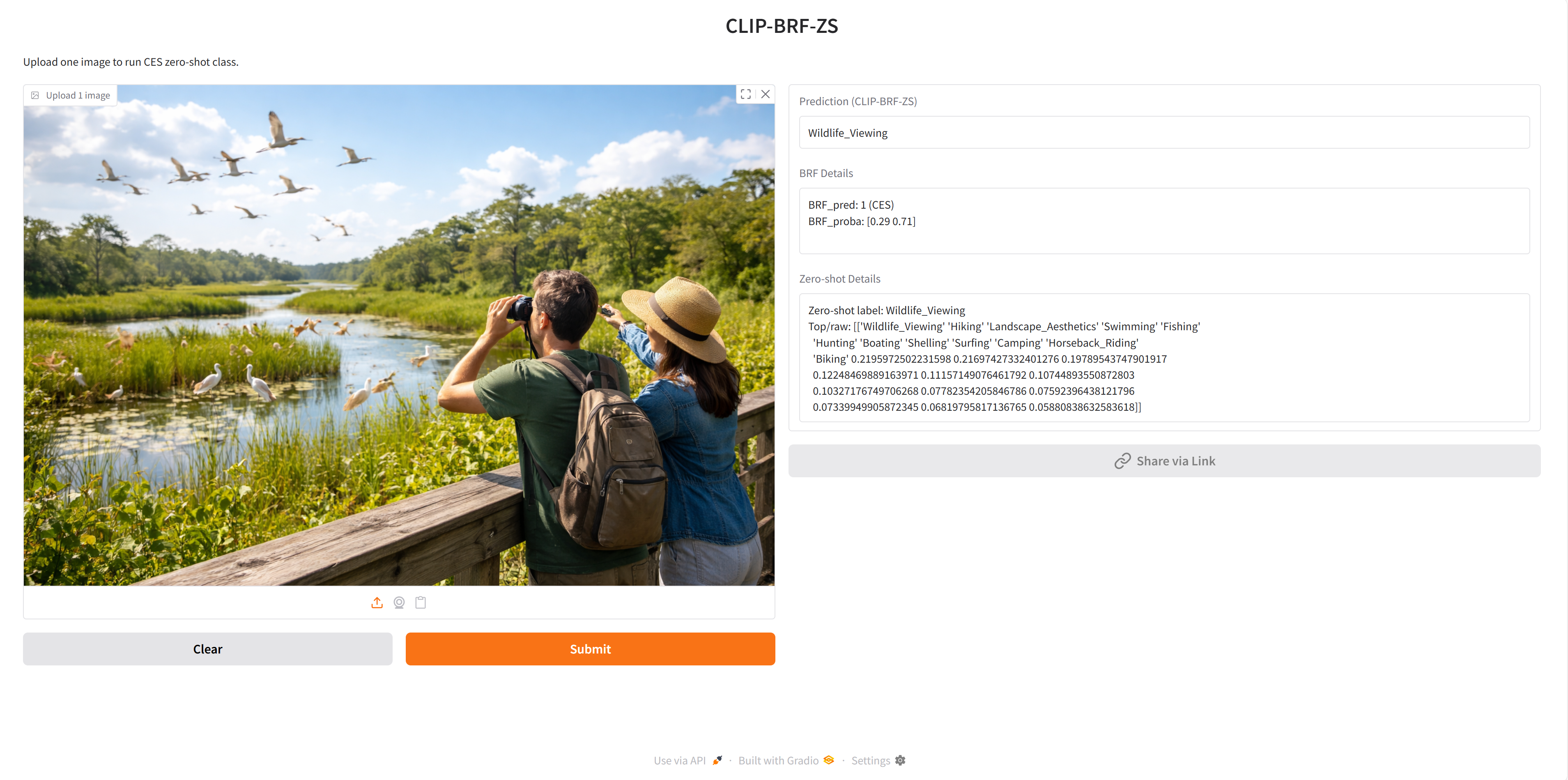
Hugging Face Application¶

🤗 Hugging Face Application: https://huggingface.co/spaces/haoyuliao/FL-CES-Flows-CLIP

Environmental Setup¶

In [1]:

!pip -q install huggingface_hub pandas pillow matplotlib
!pip -q install gdown
!pip -q install rasterio
!pip -q install geopandas folium

!pip -q install huggingface_hub pandas pillow matplotlib !pip -q install gdown !pip -q install rasterio !pip -q install geopandas folium

In [2]:

import os
import zipfile
import pandas as pd
import matplotlib.pyplot as plt
from PIL import Image
from huggingface_hub import hf_hub_download

import os import zipfile import pandas as pd import matplotlib.pyplot as plt from PIL import Image from huggingface_hub import hf_hub_download

Load Flickr30k¶

In [3]:

repo_id = "nlphuji/flickr30k"

csv_path = hf_hub_download(
    repo_id=repo_id,
    filename="flickr_annotations_30k.csv",
    repo_type="dataset"
)

zip_path = hf_hub_download(
    repo_id=repo_id,
    filename="flickr30k-images.zip",
    repo_type="dataset"
)

print("CSV downloaded to:", csv_path)
print("ZIP downloaded to:", zip_path)

repo_id = "nlphuji/flickr30k" csv_path = hf_hub_download( repo_id=repo_id, filename="flickr_annotations_30k.csv", repo_type="dataset" ) zip_path = hf_hub_download( repo_id=repo_id, filename="flickr30k-images.zip", repo_type="dataset" ) print("CSV downloaded to:", csv_path) print("ZIP downloaded to:", zip_path)

/usr/local/lib/python3.12/dist-packages/huggingface_hub/utils/_auth.py:93: UserWarning: 
The secret `HF_TOKEN` does not exist in your Colab secrets.
To authenticate with the Hugging Face Hub, create a token in your settings tab (https://huggingface.co/settings/tokens), set it as secret in your Google Colab and restart your session.
You will be able to reuse this secret in all of your notebooks.
Please note that authentication is recommended but still optional to access public models or datasets.
  warnings.warn(

CSV downloaded to: /root/.cache/huggingface/hub/datasets--nlphuji--flickr30k/snapshots/2b239befc81b6e3f035ce6bd52f5f4d60f5625f7/flickr_annotations_30k.csv
ZIP downloaded to: /root/.cache/huggingface/hub/datasets--nlphuji--flickr30k/snapshots/2b239befc81b6e3f035ce6bd52f5f4d60f5625f7/flickr30k-images.zip

Extract images¶

In [4]:

extract_dir = "/content/flickr30k_images"

if not os.path.exists(extract_dir):
    os.makedirs(extract_dir, exist_ok=True)
    with zipfile.ZipFile(zip_path, "r") as zf:
        zf.extractall(extract_dir)

print("Images extracted to:", extract_dir)

extract_dir = "/content/flickr30k_images" if not os.path.exists(extract_dir): os.makedirs(extract_dir, exist_ok=True) with zipfile.ZipFile(zip_path, "r") as zf: zf.extractall(extract_dir) print("Images extracted to:", extract_dir)

Images extracted to: /content/flickr30k_images

In [5]:

df = pd.read_csv(csv_path)
print("Data shape:", df.shape)
print(df.head())
print(df.columns)

df = pd.read_csv(csv_path) print("Data shape:", df.shape) print(df.head()) print(df.columns)

Data shape: (31014, 5)
                                                 raw               sentids  \
0  ["Two young guys with shaggy hair look at thei...       [0, 1, 2, 3, 4]   
1  ["Several men in hard hats are operating a gia...       [5, 6, 7, 8, 9]   
2  ["A child in a pink dress is climbing up a set...  [10, 11, 12, 13, 14]   
3  ["Someone in a blue shirt and hat is standing ...  [15, 16, 17, 18, 19]   
4  ["Two men, one in a gray shirt, one in a black...  [20, 21, 22, 23, 24]   

   split        filename  img_id  
0  train  1000092795.jpg       0  
1  train    10002456.jpg       1  
2  train  1000268201.jpg       2  
3  train  1000344755.jpg       3  
4  train  1000366164.jpg       4  
Index(['raw', 'sentids', 'split', 'filename', 'img_id'], dtype='object')

In [6]:

# The repo filenames are usually like "1000092795.jpg"
filename_col = "filename"   # adjust if needed after inspection
img_name = df.iloc[0][filename_col] ##Change number to check photo

# Sometimes extraction creates nested folder: /content/flickr30k_images/flickr30k-images/
candidate_paths = [
    os.path.join(extract_dir, img_name),
    os.path.join(extract_dir, "flickr30k-images", img_name),
]

img_path = None
for p in candidate_paths:
    if os.path.exists(p):
        img_path = p
        break

if img_path is None:
    raise FileNotFoundError(f"Could not find image: {img_name}")

img = Image.open(img_path)
plt.figure(figsize=(8, 6))
plt.imshow(img)
plt.axis("off")
plt.title(img_name)
plt.show()

# The repo filenames are usually like "1000092795.jpg" filename_col = "filename" # adjust if needed after inspection img_name = df.iloc[0][filename_col] ##Change number to check photo # Sometimes extraction creates nested folder: /content/flickr30k_images/flickr30k-images/ candidate_paths = [ os.path.join(extract_dir, img_name), os.path.join(extract_dir, "flickr30k-images", img_name), ] img_path = None for p in candidate_paths: if os.path.exists(p): img_path = p break if img_path is None: raise FileNotFoundError(f"Could not find image: {img_name}") img = Image.open(img_path) plt.figure(figsize=(8, 6)) plt.imshow(img) plt.axis("off") plt.title(img_name) plt.show()

CES CLIP¶

CLIP Model¶

This workshop uses CLIP (Contrastive Language–Image Pretraining) as the core vision-language model for cultural ecosystem service (CES) image classification. CLIP is designed to learn a shared embedding space for images and text, allowing visual content and natural-language descriptions to be compared directly. Instead of training a separate image classifier from scratch for each task, CLIP can perform zero-shot classification by measuring the similarity between an input image and a set of text prompts that describe possible classes.

In practice, CLIP includes two main components: an image encoder and a text encoder. The image encoder transforms an image into a numeric feature vector, while the text encoder converts each prompt into a corresponding text feature vector. These vectors are projected into the same semantic space, where similarity can be measured using cosine similarity. For a given image, the model compares its embedding with the embeddings of candidate text prompts and assigns the label associated with the most similar prompt.

This design is especially useful for CES mapping because CES categories such as biking, wildlife viewing, and landscape aesthetics can be expressed as natural-language prompts rather than requiring large task-specific training datasets. In this workshop, CLIP is used as a flexible and label-efficient foundation model for identifying CES-related content from geotagged Flickr images. The workflow builds on our recent study, which used MobileCLIP-S1 as the main CLIP variant and showed that CLIP-based approaches can provide strong CES classification performance under both closed-set and open-set conditions.

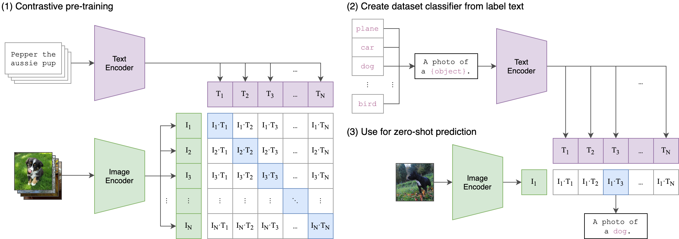Image credit from: https://github.com/openai/CLIP

Why CLIP is useful in the CES mapping¶

• It supports zero-shot learning, so categories can be defined through text prompts.
• It reduces the need for large manually labeled image datasets.
• It provides a practical way to connect social media imagery with interpretable CES categories.
• It can be combined with lightweight supervised models to improve robustness under open-set conditions.

In this notebook, CLIP is used as a practical tool for mapping CES flows from Flickr images and for demonstrating how vision-language models can support ecosystem service assessment and decision making. We will learn how to apply the CLIP-BRF-ZS tool to quantify the CES flows.

• Normalized confusion matrices for the three CLIP modeling pipelines (a) CLIP-ZS-TF, (b) CLIP-BRF-ZS, and (c) CLIP-MRF on the testing set under open-set conditions:

• Comparative performance of three CLIP-based modeling pipelines on the testing set under open-set conditions:

CLIP Environmental Setup¶

In [7]:

# =========================
# 1) Upgrade pip
# =========================
!pip -q install --upgrade pip

# =========================
# 2) Install core packages
# =========================
!pip -q install \
    numpy \
    pandas \
    scipy \
    scikit-learn \
    joblib \
    matplotlib \
    seaborn \
    openpyxl \
    geopandas \
    shapely \
    pyogrio \
    tqdm==4.67.1 \
    ftfy==6.3.1 \
    regex==2025.11.3 \
    timm==1.0.22 \
    open-clip-torch==2.29.0

# ========================= # 1) Upgrade pip # ========================= !pip -q install --upgrade pip # ========================= # 2) Install core packages # ========================= !pip -q install \ numpy \ pandas \ scipy \ scikit-learn \ joblib \ matplotlib \ seaborn \ openpyxl \ geopandas \ shapely \ pyogrio \ tqdm==4.67.1 \ ftfy==6.3.1 \ regex==2025.11.3 \ timm==1.0.22 \ open-clip-torch==2.29.0

In [8]:

# 1) Download the module file
!wget -O CLIP_Module.py "https://raw.githubusercontent.com/Ecosystem-Services-GeoAI/FL-CES-Flows-CLIP/refs/heads/main/notebooks/CLIP-BRF-ZS/CLIP_Module.py"
"""
## Helper Module: `CLIP_Module.py`

This helper module provides a set of functions used to support the **CLIP-BRF-ZS** workflow. It includes
functions for standardizing CES class names, calculating classification metrics, generating and saving
confusion matrices, loading and preprocessing images, and running CLIP-based inference on batches of
images. In practice, the module helps organize repeated tasks such as image preparation, model prediction,
and evaluation into reusable functions, making the notebook cleaner and easier to follow. The code includes
helpers such as `nameCover()` for label standardization, `classification_metrics()` for summary
statistics, `plotCom()` for confusion-matrix visualization, `storeImgs()` for image loading and
preprocessing, and `CLIP()` for batch zero-shot inference using the CLIP model.

"""
# 2) Import it
import CLIP_Module

# 3) Check available functions
print(dir(CLIP_Module))

# 1) Download the module file !wget -O CLIP_Module.py "https://raw.githubusercontent.com/Ecosystem-Services-GeoAI/FL-CES-Flows-CLIP/refs/heads/main/notebooks/CLIP-BRF-ZS/CLIP_Module.py" """ ## Helper Module: `CLIP_Module.py` This helper module provides a set of functions used to support the **CLIP-BRF-ZS** workflow. It includes functions for standardizing CES class names, calculating classification metrics, generating and saving confusion matrices, loading and preprocessing images, and running CLIP-based inference on batches of images. In practice, the module helps organize repeated tasks such as image preparation, model prediction, and evaluation into reusable functions, making the notebook cleaner and easier to follow. The code includes helpers such as `nameCover()` for label standardization, `classification_metrics()` for summary statistics, `plotCom()` for confusion-matrix visualization, `storeImgs()` for image loading and preprocessing, and `CLIP()` for batch zero-shot inference using the CLIP model. """ # 2) Import it import CLIP_Module # 3) Check available functions print(dir(CLIP_Module))

--2026-04-22 16:18:00--  https://raw.githubusercontent.com/Ecosystem-Services-GeoAI/FL-CES-Flows-CLIP/refs/heads/main/notebooks/CLIP-BRF-ZS/CLIP_Module.py
Resolving raw.githubusercontent.com (raw.githubusercontent.com)... 185.199.111.133, 185.199.108.133, 185.199.109.133, ...
Connecting to raw.githubusercontent.com (raw.githubusercontent.com)|185.199.111.133|:443... connected.
HTTP request sent, awaiting response... 200 OK
Length: 20058 (20K) [text/plain]
Saving to: ‘CLIP_Module.py’

CLIP_Module.py      100%[===================>]  19.59K  --.-KB/s    in 0.005s  

2026-04-22 16:18:00 (3.66 MB/s) - ‘CLIP_Module.py’ saved [20058/20058]

['CLIP', 'CLIP_MultPrompt', 'ConfusionMatrixDisplay', 'GetPred', 'Image', '__builtins__', '__cached__', '__doc__', '__file__', '__loader__', '__name__', '__package__', '__spec__', 'accuracy_score', 'classification_metrics', 'confusion_matrix', 'device', 'f1_score', 'hash2pandas', 'nameCover', 'np', 'os', 'pd', 'plotCom', 'plt', 'precision_score', 'recall_score', 'saveImg', 'storeImgs', 'storeImgsAllFL', 'time', 'torch']

In [9]:

import numpy as np
import torch
import warnings
import shutil
import joblib
import open_clip
from open_clip import tokenizer
import time

import os, glob
import IPython.display
import matplotlib.pyplot as plt
from PIL import Image
import numpy as np
import pandas as pd
import random

from collections import OrderedDict
import torch

import importlib

from sklearn.ensemble import RandomForestClassifier
from sklearn.metrics import classification_report, confusion_matrix
import joblib

%matplotlib inline
%config InlineBackend.figure_format = 'retina'
# Ignore all warnings5
warnings.filterwarnings("ignore")

import numpy as np import torch import warnings import shutil import joblib import open_clip from open_clip import tokenizer import time import os, glob import IPython.display import matplotlib.pyplot as plt from PIL import Image import numpy as np import pandas as pd import random from collections import OrderedDict import torch import importlib from sklearn.ensemble import RandomForestClassifier from sklearn.metrics import classification_report, confusion_matrix import joblib %matplotlib inline %config InlineBackend.figure_format = 'retina' # Ignore all warnings5 warnings.filterwarnings("ignore")

Load Module¶

In [10]:

import CLIP_Module
importlib.reload(CLIP_Module)
from CLIP_Module import *  # Re-import function to reflect updates

import CLIP_Module importlib.reload(CLIP_Module) from CLIP_Module import * # Re-import function to reflect updates

Load Images¶

In [11]:

# set your Flickr30k image folder
flickr30k_img_dir = "/content/flickr30k_images/flickr30k-images"

Florida_Images_Folders = (
    glob.glob(os.path.join(flickr30k_img_dir, "*.jpg")) +
    glob.glob(os.path.join(flickr30k_img_dir, "*.png"))
)

images_paths_map = {
    os.path.basename(x).split(".")[0]: x
    for x in Florida_Images_Folders
}

photo_ids = [
    os.path.basename(x).split(".")[0]
    for x in Florida_Images_Folders
]



random.seed(119)
photo_ids = random.sample(photo_ids, 5)
print("Number of images:", len(Florida_Images_Folders))
print("Example photo id:", photo_ids[:5])

# set your Flickr30k image folder flickr30k_img_dir = "/content/flickr30k_images/flickr30k-images" Florida_Images_Folders = ( glob.glob(os.path.join(flickr30k_img_dir, "*.jpg")) + glob.glob(os.path.join(flickr30k_img_dir, "*.png")) ) images_paths_map = { os.path.basename(x).split(".")[0]: x for x in Florida_Images_Folders } photo_ids = [ os.path.basename(x).split(".")[0] for x in Florida_Images_Folders ] random.seed(119) photo_ids = random.sample(photo_ids, 5) print("Number of images:", len(Florida_Images_Folders)) print("Example photo id:", photo_ids[:5])

Number of images: 31783
Example photo id: ['67491882', '2366020313', '4986921677', '2563043367', '6939568656']

In [12]:

import matplotlib.pyplot as plt
from PIL import Image

# show selected 5 images
fig, axes = plt.subplots(1, len(photo_ids), figsize=(20, 5))

if len(photo_ids) == 1:
    axes = [axes]

for ax, pid in zip(axes, photo_ids):
    img_path = images_paths_map[pid]
    img = Image.open(img_path)
    ax.imshow(img)
    ax.set_title(pid, fontsize=10)
    ax.axis("off")

plt.tight_layout()
plt.show()

import matplotlib.pyplot as plt from PIL import Image # show selected 5 images fig, axes = plt.subplots(1, len(photo_ids), figsize=(20, 5)) if len(photo_ids) == 1: axes = [axes] for ax, pid in zip(axes, photo_ids): img_path = images_paths_map[pid] img = Image.open(img_path) ax.imshow(img) ax.set_title(pid, fontsize=10) ax.axis("off") plt.tight_layout() plt.show()

Load the trained Binary Random Forest (BRF) model¶

Binary Random Forest (BRF) Model¶

In this workflow, the Binary Random Forest (BRF) model is used as a first-level filtering step to distinguish CES-relevant images from irrelevant or out-of-scope images. Random Forest is an ensemble learning method that fits multiple decision trees on bootstrap samples and combines their predictions to improve robustness and generalization. Here, we use the scikit-learn implementation of RandomForestClassifier to train the BRF on CLIP-derived image embeddings.

After training, the fitted BRF model is saved and later loaded as a pretrained model object using joblib.load(), which is a common way to serialize and reuse scikit-learn models in Python. This allows the workshop workflow to apply the trained BRF directly without retraining it each time. See the official documentation for scikit-learn RandomForestClassifier.

Image logo from: https://scikit-learn.org/

In [13]:

!wget -O BRF_model.joblib "https://raw.githubusercontent.com/Ecosystem-Services-GeoAI/FL-CES-Flows-CLIP/main/model/BRF_model.joblib"

!wget -O BRF_model.joblib "https://raw.githubusercontent.com/Ecosystem-Services-GeoAI/FL-CES-Flows-CLIP/main/model/BRF_model.joblib"

--2026-04-22 16:18:48--  https://raw.githubusercontent.com/Ecosystem-Services-GeoAI/FL-CES-Flows-CLIP/main/model/BRF_model.joblib
Resolving raw.githubusercontent.com (raw.githubusercontent.com)... 185.199.108.133, 185.199.109.133, 185.199.110.133, ...
Connecting to raw.githubusercontent.com (raw.githubusercontent.com)|185.199.108.133|:443... connected.
HTTP request sent, awaiting response... 200 OK
Length: 517449 (505K) [application/octet-stream]
Saving to: ‘BRF_model.joblib’

BRF_model.joblib    100%[===================>] 505.32K  --.-KB/s    in 0.1s    

2026-04-22 16:18:49 (4.01 MB/s) - ‘BRF_model.joblib’ saved [517449/517449]

In [14]:

clf = joblib.load("BRF_model.joblib")

clf = joblib.load("BRF_model.joblib")

Load CLIP model¶

In [15]:

# Load CLIP Model
model_name = 'MobileCLIP-S1'  # Replace with your model
pretrained = 'datacompdr'      # Specify the pretrained source
model, _, preprocess = open_clip.create_model_and_transforms(model_name, pretrained=pretrained)
tokenizer = open_clip.get_tokenizer(model_name)  # Correct tokenizer initialization

# Set device
device = "cuda" if torch.cuda.is_available() else "cpu"
model.to(device)
model.eval(); #Important to turn on.

# Load CLIP Model model_name = 'MobileCLIP-S1' # Replace with your model pretrained = 'datacompdr' # Specify the pretrained source model, _, preprocess = open_clip.create_model_and_transforms(model_name, pretrained=pretrained) tokenizer = open_clip.get_tokenizer(model_name) # Correct tokenizer initialization # Set device device = "cuda" if torch.cuda.is_available() else "cpu" model.to(device) model.eval(); #Important to turn on.

Available CLIP Models¶

The current open_clip environment provides 163 available model–checkpoint combinations that can be used for inference. Each option is defined by a pair of values: model_name and pretrained. The model_name specifies the CLIP architecture or backbone, while pretrained specifies which pretrained checkpoint is loaded for that architecture. Together, these two settings determine which vision-language model is used in the workflow. The detailed pretrain list

You can change the parameters below to load a different CLIP model.

model_name = " "
pretrained = " "

In [16]:

from IPython.display import HTML
pairs = open_clip.list_pretrained()
df_models = pd.DataFrame(pairs, columns=["model_name", "pretrained"])

html = df_models.to_html()
HTML(f"""
<h2>Available CLIP Models</h2>
<div style="max-height:600px; overflow:auto; border:1px solid #ccc;">
{html}
</div>
""")

from IPython.display import HTML pairs = open_clip.list_pretrained() df_models = pd.DataFrame(pairs, columns=["model_name", "pretrained"]) html = df_models.to_html() HTML(f""" <h2>Available CLIP Models</h2> <div style="max-height:600px; overflow:auto; border:1px solid #ccc;"> {html} </div> """)

Out[16]:

Available CLIP Models

	model_name	pretrained
0	RN50	openai
1	RN50	yfcc15m
2	RN50	cc12m
3	RN101	openai
4	RN101	yfcc15m
5	RN50x4	openai
6	RN50x16	openai
7	RN50x64	openai
8	ViT-B-32	openai
9	ViT-B-32	laion400m_e31
10	ViT-B-32	laion400m_e32
11	ViT-B-32	laion2b_e16
12	ViT-B-32	laion2b_s34b_b79k
13	ViT-B-32	datacomp_xl_s13b_b90k
14	ViT-B-32	datacomp_m_s128m_b4k
15	ViT-B-32	commonpool_m_clip_s128m_b4k
16	ViT-B-32	commonpool_m_laion_s128m_b4k
17	ViT-B-32	commonpool_m_image_s128m_b4k
18	ViT-B-32	commonpool_m_text_s128m_b4k
19	ViT-B-32	commonpool_m_basic_s128m_b4k
20	ViT-B-32	commonpool_m_s128m_b4k
21	ViT-B-32	datacomp_s_s13m_b4k
22	ViT-B-32	commonpool_s_clip_s13m_b4k
23	ViT-B-32	commonpool_s_laion_s13m_b4k
24	ViT-B-32	commonpool_s_image_s13m_b4k
25	ViT-B-32	commonpool_s_text_s13m_b4k
26	ViT-B-32	commonpool_s_basic_s13m_b4k
27	ViT-B-32	commonpool_s_s13m_b4k
28	ViT-B-32	metaclip_400m
29	ViT-B-32	metaclip_fullcc
30	ViT-B-32-256	datacomp_s34b_b86k
31	ViT-B-16	openai
32	ViT-B-16	laion400m_e31
33	ViT-B-16	laion400m_e32
34	ViT-B-16	laion2b_s34b_b88k
35	ViT-B-16	datacomp_xl_s13b_b90k
36	ViT-B-16	datacomp_l_s1b_b8k
37	ViT-B-16	commonpool_l_clip_s1b_b8k
38	ViT-B-16	commonpool_l_laion_s1b_b8k
39	ViT-B-16	commonpool_l_image_s1b_b8k
40	ViT-B-16	commonpool_l_text_s1b_b8k
41	ViT-B-16	commonpool_l_basic_s1b_b8k
42	ViT-B-16	commonpool_l_s1b_b8k
43	ViT-B-16	dfn2b
44	ViT-B-16	metaclip_400m
45	ViT-B-16	metaclip_fullcc
46	ViT-B-16-plus-240	laion400m_e31
47	ViT-B-16-plus-240	laion400m_e32
48	ViT-L-14	openai
49	ViT-L-14	laion400m_e31
50	ViT-L-14	laion400m_e32
51	ViT-L-14	laion2b_s32b_b82k
52	ViT-L-14	datacomp_xl_s13b_b90k
53	ViT-L-14	commonpool_xl_clip_s13b_b90k
54	ViT-L-14	commonpool_xl_laion_s13b_b90k
55	ViT-L-14	commonpool_xl_s13b_b90k
56	ViT-L-14	metaclip_400m
57	ViT-L-14	metaclip_fullcc
58	ViT-L-14	dfn2b
59	ViT-L-14-336	openai
60	ViT-H-14	laion2b_s32b_b79k
61	ViT-H-14	metaclip_fullcc
62	ViT-H-14	dfn5b
63	ViT-H-14-378	dfn5b
64	ViT-g-14	laion2b_s12b_b42k
65	ViT-g-14	laion2b_s34b_b88k
66	ViT-bigG-14	laion2b_s39b_b160k
67	ViT-bigG-14	metaclip_fullcc
68	roberta-ViT-B-32	laion2b_s12b_b32k
69	xlm-roberta-base-ViT-B-32	laion5b_s13b_b90k
70	xlm-roberta-large-ViT-H-14	frozen_laion5b_s13b_b90k
71	convnext_base	laion400m_s13b_b51k
72	convnext_base_w	laion2b_s13b_b82k
73	convnext_base_w	laion2b_s13b_b82k_augreg
74	convnext_base_w	laion_aesthetic_s13b_b82k
75	convnext_base_w_320	laion_aesthetic_s13b_b82k
76	convnext_base_w_320	laion_aesthetic_s13b_b82k_augreg
77	convnext_large_d	laion2b_s26b_b102k_augreg
78	convnext_large_d_320	laion2b_s29b_b131k_ft
79	convnext_large_d_320	laion2b_s29b_b131k_ft_soup
80	convnext_xxlarge	laion2b_s34b_b82k_augreg
81	convnext_xxlarge	laion2b_s34b_b82k_augreg_rewind
82	convnext_xxlarge	laion2b_s34b_b82k_augreg_soup
83	coca_ViT-B-32	laion2b_s13b_b90k
84	coca_ViT-B-32	mscoco_finetuned_laion2b_s13b_b90k
85	coca_ViT-L-14	laion2b_s13b_b90k
86	coca_ViT-L-14	mscoco_finetuned_laion2b_s13b_b90k
87	EVA01-g-14	laion400m_s11b_b41k
88	EVA01-g-14-plus	merged2b_s11b_b114k
89	EVA02-B-16	merged2b_s8b_b131k
90	EVA02-L-14	merged2b_s4b_b131k
91	EVA02-L-14-336	merged2b_s6b_b61k
92	EVA02-E-14	laion2b_s4b_b115k
93	EVA02-E-14-plus	laion2b_s9b_b144k
94	ViT-B-16-SigLIP	webli
95	ViT-B-16-SigLIP-256	webli
96	ViT-B-16-SigLIP-i18n-256	webli
97	ViT-B-16-SigLIP-384	webli
98	ViT-B-16-SigLIP-512	webli
99	ViT-L-16-SigLIP-256	webli
100	ViT-L-16-SigLIP-384	webli
101	ViT-SO400M-14-SigLIP	webli
102	ViT-SO400M-16-SigLIP-i18n-256	webli
103	ViT-SO400M-14-SigLIP-378	webli
104	ViT-SO400M-14-SigLIP-384	webli
105	ViT-L-14-CLIPA	datacomp1b
106	ViT-L-14-CLIPA-336	datacomp1b
107	ViT-H-14-CLIPA	datacomp1b
108	ViT-H-14-CLIPA-336	laion2b
109	ViT-H-14-CLIPA-336	datacomp1b
110	ViT-bigG-14-CLIPA	datacomp1b
111	ViT-bigG-14-CLIPA-336	datacomp1b
112	nllb-clip-base	v1
113	nllb-clip-large	v1
114	nllb-clip-base-siglip	v1
115	nllb-clip-base-siglip	mrl
116	nllb-clip-large-siglip	v1
117	nllb-clip-large-siglip	mrl
118	MobileCLIP-S1	datacompdr
119	MobileCLIP-S2	datacompdr
120	MobileCLIP-B	datacompdr
121	MobileCLIP-B	datacompdr_lt
122	ViTamin-S	datacomp1b
123	ViTamin-S-LTT	datacomp1b
124	ViTamin-B	datacomp1b
125	ViTamin-B-LTT	datacomp1b
126	ViTamin-L	datacomp1b
127	ViTamin-L-256	datacomp1b
128	ViTamin-L-336	datacomp1b
129	ViTamin-L-384	datacomp1b
130	ViTamin-L2	datacomp1b
131	ViTamin-L2-256	datacomp1b
132	ViTamin-L2-336	datacomp1b
133	ViTamin-L2-384	datacomp1b
134	ViTamin-XL-256	datacomp1b
135	ViTamin-XL-336	datacomp1b
136	ViTamin-XL-384	datacomp1b
137	RN50-quickgelu	openai
138	RN50-quickgelu	yfcc15m
139	RN50-quickgelu	cc12m
140	RN101-quickgelu	openai
141	RN101-quickgelu	yfcc15m
142	RN50x4-quickgelu	openai
143	RN50x16-quickgelu	openai
144	RN50x64-quickgelu	openai
145	ViT-B-32-quickgelu	openai
146	ViT-B-32-quickgelu	laion400m_e31
147	ViT-B-32-quickgelu	laion400m_e32
148	ViT-B-32-quickgelu	metaclip_400m
149	ViT-B-32-quickgelu	metaclip_fullcc
150	ViT-B-16-quickgelu	openai
151	ViT-B-16-quickgelu	dfn2b
152	ViT-B-16-quickgelu	metaclip_400m
153	ViT-B-16-quickgelu	metaclip_fullcc
154	ViT-L-14-quickgelu	openai
155	ViT-L-14-quickgelu	metaclip_400m
156	ViT-L-14-quickgelu	metaclip_fullcc
157	ViT-L-14-quickgelu	dfn2b
158	ViT-L-14-336-quickgelu	openai
159	ViT-H-14-quickgelu	metaclip_fullcc
160	ViT-H-14-quickgelu	dfn5b
161	ViT-H-14-378-quickgelu	dfn5b
162	ViT-bigG-14-quickgelu	metaclip_fullcc

Pretrained tag	What it refers to	Dataset type / content	Dataset / source link
openai	OpenAI’s original CLIP checkpoint, associated with WIT / WebImageText in the OpenCLIP README.	Large-scale web image–text pairs collected from the web; general-purpose image–caption style pretraining.	OpenCLIP README
yfcc15m	A checkpoint trained on YFCC15M, derived from Flickr Creative Commons imagery.	Social media / photo-sharing imagery from Flickr with metadata; broad real-world photography, places, events, people, nature, etc.	YFCC100M overview
cc12m	A checkpoint trained on Conceptual 12M (CC12M).	Large-scale web image–caption pairs collected for vision–language pretraining; broad visual concepts rather than a specific domain such as animals only.	Conceptual 12M
laion400m_*	Checkpoints trained on LAION-400M variants.	Large-scale web-scale image–text pairs filtered with CLIP; broad open-domain internet imagery.	LAION-400M
laion2b_*	Checkpoints trained on LAION-2B variants.	Very large-scale web image–text pairs from the LAION-5B family; broad open-domain internet imagery.	LAION-5B / LAION-2B
datacomp* / datacomp1b / datacompdr	Checkpoints associated with DataComp training data or DataComp-derived recipes.	Benchmark-oriented web image–text datasets designed to compare data selection strategies for multimodal training.	DataComp
metaclip_*	Checkpoints associated with MetaCLIP training data.	Large-scale web image–text data assembled for contrastive pretraining; broad general-purpose vision–language learning.	MetaCLIP repository
webli	Checkpoints trained with WebLI data.	Large multilingual web image–language pairs used by Google for vision–language pretraining.	PaLI / WebLI
dfn2b, dfn5b	Checkpoints associated with DFN-2B and DFN-5B training data.	Large-scale filtered web image–text datasets built with data filtering strategies for CLIP-style training.	DFN paper

BRF First-Level Inference¶

In this workflow, the Binary Random Forest (BRF) serves as the first-level inference step in the CLIP-BRF-ZS pipeline. Its role is to act as a lightweight filter that separates CES-relevant images from irrelevant or out-of-scope images before the zero-shot CLIP classification stage. Rather than asking CLIP to classify every Flickr image directly into the target CES classes, the BRF first screens the input using CLIP-derived image embeddings and predicts whether an image belongs to the targeted CES content or should be assigned to the “other” category. Images predicted as irrelevant are excluded from further CES classification, while images predicted as relevant are passed to the second stage, where CLIP assigns one of the CES class labels using text prompts.

This two-stage design helps reduce false assignments caused by noisy social media imagery and improves robustness under open-set conditions. In our Florida case study, this hybrid filtering strategy substantially improved performance compared with zero-shot threshold filtering alone and fully supervised multiclass classification under low-label conditions.

In [17]:

import psutil

y_pred = []
images = []
images_valid = [] #1 valid; 0: corruption
start_time = time.perf_counter()
n = 1

sub_start_time = time.perf_counter()
for idx in range(len(photo_ids)):
    try:
        image_path = images_paths_map[str(photo_ids[idx])]
        image = Image.open(image_path).convert("RGB")
        images_valid.append(1)
    except:
        image_path = images_paths_map[str(photo_ids[0])] #Fake Image
        image = Image.open(image_path).convert("RGB")
        images_valid.append(0)

    images.append(preprocess(image).to(device))

    if (idx+1)%500 == 0 or (idx+1) == len(photo_ids):
        image_input = torch.stack(images).to(device)
        with torch.no_grad():
            image_features = model.encode_image(image_input).float()

        image_features_cpu = np.array(image_features.cpu())

        pred = clf.predict(image_features_cpu) #RF prediciton
        y_pred.append(pred)

        del image_input, image_features, images, image_features_cpu
        torch.cuda.empty_cache()  # Clear unused memory
        images = []

        # Get the memory usage in bytes
        memory_usage = psutil.Process().memory_info().rss

        # Convert to megabytes
        memory_usage_mb = memory_usage / (1024 ** 2)

        # End the timer
        sub_end_time = time.perf_counter()
        # Calculate the time taken
        sub_execution_time = sub_end_time - sub_start_time
        sub_start_time = time.perf_counter()
        print(f"{n} Execution time: {sub_execution_time:.6f} seconds")
        print(f"Memory Usage: {memory_usage_mb:.2f} MB")
        n+=1

y_pred_flat = np.concatenate(y_pred) #1: CES; 0:Other

import psutil y_pred = [] images = [] images_valid = [] #1 valid; 0: corruption start_time = time.perf_counter() n = 1 sub_start_time = time.perf_counter() for idx in range(len(photo_ids)): try: image_path = images_paths_map[str(photo_ids[idx])] image = Image.open(image_path).convert("RGB") images_valid.append(1) except: image_path = images_paths_map[str(photo_ids[0])] #Fake Image image = Image.open(image_path).convert("RGB") images_valid.append(0) images.append(preprocess(image).to(device)) if (idx+1)%500 == 0 or (idx+1) == len(photo_ids): image_input = torch.stack(images).to(device) with torch.no_grad(): image_features = model.encode_image(image_input).float() image_features_cpu = np.array(image_features.cpu()) pred = clf.predict(image_features_cpu) #RF prediciton y_pred.append(pred) del image_input, image_features, images, image_features_cpu torch.cuda.empty_cache() # Clear unused memory images = [] # Get the memory usage in bytes memory_usage = psutil.Process().memory_info().rss # Convert to megabytes memory_usage_mb = memory_usage / (1024 ** 2) # End the timer sub_end_time = time.perf_counter() # Calculate the time taken sub_execution_time = sub_end_time - sub_start_time sub_start_time = time.perf_counter() print(f"{n} Execution time: {sub_execution_time:.6f} seconds") print(f"Memory Usage: {memory_usage_mb:.2f} MB") n+=1 y_pred_flat = np.concatenate(y_pred) #1: CES; 0:Other

1 Execution time: 8.587920 seconds
Memory Usage: 1085.72 MB

CLIP second level inference¶

In [18]:

descriptions = {
    "Hiking": "This is an image of people hiking or taking a casual walk on challenging scenic trails or through breathtaking countryside.",
    "Boating": "This is an image of boating with powerboats or human-powered vessels such as rowboats or paddle boats.",
    "Swimming":"This is an image of people wearing swimsuits while swimming in a pool, lake, or ocean.",
    "Camping":"This is camping.",
    "Fishing":"This is fishing.",
    "Biking":"This is biking.",
    "Horseback_Riding":"This is horseback riding.",
    "Wildlife_Viewing":"This is an image without people, showing wildlife such as birds, flowers, or fungi in a natural environment.",
    "Shelling":"This is shelling.",
    "Surfing": "This is an image of people surfing on ocean waves or holding a surfboard on the beach.",
    "Hunting": "This is an image of a hunter posing with a large kill, cleaning or gutting the carcass of a feral animal.",
    "Landscape_Aesthetics":"This is an image without people, showing a natural, soothing, and vibrant panoramic landscape."
}

class_names = ["Hiking", "Boating", "Swimming", "Camping", "Fishing", "Biking", "Horseback_Riding", "Wildlife_Viewing",
              "Shelling", "Surfing", "Hunting","Landscape_Aesthetics"]

texts = []
for name in descriptions:
    texts.append(descriptions[name])


text_tokens = tokenizer([desc for desc in texts]).to(device)


images = []
images_valid = [] #1: valid; 0: corruption
original_images = []
predicted_cover_labels_col = []

# Start the timer
start_time = time.perf_counter()
n = 1
for idx in range(len(photo_ids)):
    sub_start_time = time.perf_counter()

    try:
        image_path = images_paths_map[str(photo_ids[idx])]
        image = Image.open(image_path).convert("RGB")
        images_valid.append(1)
    except:
        image_path = images_paths_map[str(photo_ids[0])] #Fake Image
        image = Image.open(image_path).convert("RGB")
        images_valid.append(0)
        continue

    images.append(preprocess(image).to(device))

    if (idx+1)%500 == 0 or (idx+1) == len(photo_ids):
        image_input = torch.stack(images).to(device)
        with torch.no_grad():
            image_features = model.encode_image(image_input).float()
            text_features = model.encode_text(text_tokens).float()

        image_features /= image_features.norm(dim=-1, keepdim=True)
        text_features /= text_features.norm(dim=-1, keepdim=True)
        subsimilarity = text_features.cpu().numpy() @ image_features.cpu().numpy().T
        predicted_cover_labels, top = GetPred(subsimilarity, class_names)
        predicted_cover_labels_col += predicted_cover_labels

        if n == 1:
            tops = top.copy()
        else:
            tops = np.vstack((tops, top.copy()))

        n+=1

        del image_input, image_features, text_features, subsimilarity, images, predicted_cover_labels, top
        torch.cuda.empty_cache()  # Clear unused memory
        images = []

        # End the timer
        sub_end_time = time.perf_counter()
        # Calculate the time taken
        sub_execution_time = sub_end_time - sub_start_time
        print(f"{n} Execution time: {sub_execution_time:.6f} seconds")

# End the timer
end_time = time.perf_counter()
# Calculate the time taken
execution_time = end_time - start_time
print(f"Execution time: {execution_time:.6f} seconds")

descriptions = { "Hiking": "This is an image of people hiking or taking a casual walk on challenging scenic trails or through breathtaking countryside.", "Boating": "This is an image of boating with powerboats or human-powered vessels such as rowboats or paddle boats.", "Swimming":"This is an image of people wearing swimsuits while swimming in a pool, lake, or ocean.", "Camping":"This is camping.", "Fishing":"This is fishing.", "Biking":"This is biking.", "Horseback_Riding":"This is horseback riding.", "Wildlife_Viewing":"This is an image without people, showing wildlife such as birds, flowers, or fungi in a natural environment.", "Shelling":"This is shelling.", "Surfing": "This is an image of people surfing on ocean waves or holding a surfboard on the beach.", "Hunting": "This is an image of a hunter posing with a large kill, cleaning or gutting the carcass of a feral animal.", "Landscape_Aesthetics":"This is an image without people, showing a natural, soothing, and vibrant panoramic landscape." } class_names = ["Hiking", "Boating", "Swimming", "Camping", "Fishing", "Biking", "Horseback_Riding", "Wildlife_Viewing", "Shelling", "Surfing", "Hunting","Landscape_Aesthetics"] texts = [] for name in descriptions: texts.append(descriptions[name]) text_tokens = tokenizer([desc for desc in texts]).to(device) images = [] images_valid = [] #1: valid; 0: corruption original_images = [] predicted_cover_labels_col = [] # Start the timer start_time = time.perf_counter() n = 1 for idx in range(len(photo_ids)): sub_start_time = time.perf_counter() try: image_path = images_paths_map[str(photo_ids[idx])] image = Image.open(image_path).convert("RGB") images_valid.append(1) except: image_path = images_paths_map[str(photo_ids[0])] #Fake Image image = Image.open(image_path).convert("RGB") images_valid.append(0) continue images.append(preprocess(image).to(device)) if (idx+1)%500 == 0 or (idx+1) == len(photo_ids): image_input = torch.stack(images).to(device) with torch.no_grad(): image_features = model.encode_image(image_input).float() text_features = model.encode_text(text_tokens).float() image_features /= image_features.norm(dim=-1, keepdim=True) text_features /= text_features.norm(dim=-1, keepdim=True) subsimilarity = text_features.cpu().numpy() @ image_features.cpu().numpy().T predicted_cover_labels, top = GetPred(subsimilarity, class_names) predicted_cover_labels_col += predicted_cover_labels if n == 1: tops = top.copy() else: tops = np.vstack((tops, top.copy())) n+=1 del image_input, image_features, text_features, subsimilarity, images, predicted_cover_labels, top torch.cuda.empty_cache() # Clear unused memory images = [] # End the timer sub_end_time = time.perf_counter() # Calculate the time taken sub_execution_time = sub_end_time - sub_start_time print(f"{n} Execution time: {sub_execution_time:.6f} seconds") # End the timer end_time = time.perf_counter() # Calculate the time taken execution_time = end_time - start_time print(f"Execution time: {execution_time:.6f} seconds")

2 Execution time: 11.749081 seconds
Execution time: 11.892157 seconds

Outcomes¶

In [19]:

res = {
    "pid": [],
    "CLIP-BRF-ZS": [],
    "Image_Path": []
}

for i, pid in enumerate(photo_ids):
    res["pid"].append(pid)

    label = (
        predicted_cover_labels_col[i]
        if y_pred_flat[i] == 1
        else "Other"
    )
    res["CLIP-BRF-ZS"].append(label)

    res["Image_Path"].append(images_paths_map.get(pid, None))


df_res = pd.DataFrame(res)
df_res.to_csv("df_res.csv", index=False)

res = { "pid": [], "CLIP-BRF-ZS": [], "Image_Path": [] } for i, pid in enumerate(photo_ids): res["pid"].append(pid) label = ( predicted_cover_labels_col[i] if y_pred_flat[i] == 1 else "Other" ) res["CLIP-BRF-ZS"].append(label) res["Image_Path"].append(images_paths_map.get(pid, None)) df_res = pd.DataFrame(res) df_res.to_csv("df_res.csv", index=False)

In [20]:

# from google.colab import files
# df_res.to_csv("/content/df_res.csv", index=False)
# files.download("/content/df_res.csv")

# from google.colab import files # df_res.to_csv("/content/df_res.csv", index=False) # files.download("/content/df_res.csv")

Example Outputs¶

In [21]:

for i in range(5):
    img = Image.open(df_res.loc[i, "Image_Path"])

    plt.figure(figsize=(4, 4))
    plt.imshow(img)
    plt.axis("off")

    title = f"""
    PID: {df_res.loc[i, 'pid']}
    Prediction: {df_res.loc[i, 'CLIP-BRF-ZS']}
    """
    plt.title(title.strip(), fontsize=10)
    plt.show()

for i in range(5): img = Image.open(df_res.loc[i, "Image_Path"]) plt.figure(figsize=(4, 4)) plt.imshow(img) plt.axis("off") title = f""" PID: {df_res.loc[i, 'pid']} Prediction: {df_res.loc[i, 'CLIP-BRF-ZS']} """ plt.title(title.strip(), fontsize=10) plt.show()

Spatial Analysis PUDs¶

Defining CES Flow Metrics: PUD as a Proxy¶

In this workshop, we use photo-user-days (PUDs) as a proxy for cultural ecosystem service (CES) flows derived from geotagged Flickr images. A PUD represents the number of unique users who took at least one photograph in a given location on a given day. This metric is commonly used in social-media-based recreation and CES studies because it reduces bias from highly active users who may upload many images during a single visit. Instead of counting raw photo numbers, PUDs provide a more stable proxy for visitation intensity and realized human–nature interactions.

In this notebook, we use two related CES flow metrics:

1. Average annual PUDs, denoted as $\overline{PUD}_{yr}$
   This metric measures the average annual number of photo-user-days for a CES class within a 1 km grid cell. It represents the total magnitude of CES flow at a location and helps identify where overall human engagement with landscapes is highest.

   

2. Average annual PUDs per user, denoted as $\overline{PUD}_{user,yr}$
   This metric standardizes $\overline{PUD}_{yr}$ by the total number of unique users in the study period. It represents per-user flow intensity and allows comparison of how strongly individuals engage with CES across landscape types, independent of overall user volume.

   

where i denotes the 1 km grid cell, c denotes the CES class, and N_user denotes the total number of unique users contributing geotagged images during the study period.

Together, these two metrics help us examine both the overall volume of CES flows and the intensity of engagement per user across Florida’s natural and working lands.

In [22]:

import pandas as pd
import geopandas as gpd
from shapely.geometry import Point
import matplotlib.pyplot as plt
import os

import pandas as pd import geopandas as gpd from shapely.geometry import Point import matplotlib.pyplot as plt import os

Data Preparation¶

In [23]:

# make folders
!mkdir -p /content/model-outputs/FL_1km_Grid

# download shapefile components
!wget -O /content/model-outputs/FL_1km_Grid/FL_1km_Grid.shp "https://raw.githubusercontent.com/Ecosystem-Services-GeoAI/FL-CES-Flows-CLIP/main/model-outputs/FL_1km_Grid/FL_1km_Grid.shp"
!wget -O /content/model-outputs/FL_1km_Grid/FL_1km_Grid.shx "https://raw.githubusercontent.com/Ecosystem-Services-GeoAI/FL-CES-Flows-CLIP/main/model-outputs/FL_1km_Grid/FL_1km_Grid.shx"
!wget -O /content/model-outputs/FL_1km_Grid/FL_1km_Grid.dbf "https://raw.githubusercontent.com/Ecosystem-Services-GeoAI/FL-CES-Flows-CLIP/main/model-outputs/FL_1km_Grid/FL_1km_Grid.dbf"
!wget -O /content/model-outputs/FL_1km_Grid/FL_1km_Grid.prj "https://raw.githubusercontent.com/Ecosystem-Services-GeoAI/FL-CES-Flows-CLIP/main/model-outputs/FL_1km_Grid/FL_1km_Grid.prj"
!wget -O /content/model-outputs/FL_1km_Grid/FL_1km_Grid.cpg "https://raw.githubusercontent.com/Ecosystem-Services-GeoAI/FL-CES-Flows-CLIP/main/model-outputs/FL_1km_Grid/FL_1km_Grid.cpg"

# download metadata csv
!wget -O /content/model-outputs/Flickr_FL_Predictions_2014_2019_CLIP-BRF-ZS.csv "https://raw.githubusercontent.com/Ecosystem-Services-GeoAI/FL-CES-Flows-CLIP/main/model-outputs/Flickr_FL_Predictions_2014_2019_CLIP-BRF-ZS.csv"

# make folders !mkdir -p /content/model-outputs/FL_1km_Grid # download shapefile components !wget -O /content/model-outputs/FL_1km_Grid/FL_1km_Grid.shp "https://raw.githubusercontent.com/Ecosystem-Services-GeoAI/FL-CES-Flows-CLIP/main/model-outputs/FL_1km_Grid/FL_1km_Grid.shp" !wget -O /content/model-outputs/FL_1km_Grid/FL_1km_Grid.shx "https://raw.githubusercontent.com/Ecosystem-Services-GeoAI/FL-CES-Flows-CLIP/main/model-outputs/FL_1km_Grid/FL_1km_Grid.shx" !wget -O /content/model-outputs/FL_1km_Grid/FL_1km_Grid.dbf "https://raw.githubusercontent.com/Ecosystem-Services-GeoAI/FL-CES-Flows-CLIP/main/model-outputs/FL_1km_Grid/FL_1km_Grid.dbf" !wget -O /content/model-outputs/FL_1km_Grid/FL_1km_Grid.prj "https://raw.githubusercontent.com/Ecosystem-Services-GeoAI/FL-CES-Flows-CLIP/main/model-outputs/FL_1km_Grid/FL_1km_Grid.prj" !wget -O /content/model-outputs/FL_1km_Grid/FL_1km_Grid.cpg "https://raw.githubusercontent.com/Ecosystem-Services-GeoAI/FL-CES-Flows-CLIP/main/model-outputs/FL_1km_Grid/FL_1km_Grid.cpg" # download metadata csv !wget -O /content/model-outputs/Flickr_FL_Predictions_2014_2019_CLIP-BRF-ZS.csv "https://raw.githubusercontent.com/Ecosystem-Services-GeoAI/FL-CES-Flows-CLIP/main/model-outputs/Flickr_FL_Predictions_2014_2019_CLIP-BRF-ZS.csv"

--2026-04-22 16:19:22--  https://raw.githubusercontent.com/Ecosystem-Services-GeoAI/FL-CES-Flows-CLIP/main/model-outputs/FL_1km_Grid/FL_1km_Grid.shp
Resolving raw.githubusercontent.com (raw.githubusercontent.com)... 185.199.108.133, 185.199.109.133, 185.199.110.133, ...
Connecting to raw.githubusercontent.com (raw.githubusercontent.com)|185.199.108.133|:443... connected.
HTTP request sent, awaiting response... 200 OK
Length: 25761244 (25M) [application/octet-stream]
Saving to: ‘/content/model-outputs/FL_1km_Grid/FL_1km_Grid.shp’

/content/model-outp 100%[===================>]  24.57M  56.9MB/s    in 0.4s    

2026-04-22 16:19:24 (56.9 MB/s) - ‘/content/model-outputs/FL_1km_Grid/FL_1km_Grid.shp’ saved [25761244/25761244]

--2026-04-22 16:19:25--  https://raw.githubusercontent.com/Ecosystem-Services-GeoAI/FL-CES-Flows-CLIP/main/model-outputs/FL_1km_Grid/FL_1km_Grid.shx
Resolving raw.githubusercontent.com (raw.githubusercontent.com)... 185.199.109.133, 185.199.111.133, 185.199.108.133, ...
Connecting to raw.githubusercontent.com (raw.githubusercontent.com)|185.199.109.133|:443... connected.
HTTP request sent, awaiting response... 200 OK
Length: 1495892 (1.4M) [application/octet-stream]
Saving to: ‘/content/model-outputs/FL_1km_Grid/FL_1km_Grid.shx’

/content/model-outp 100%[===================>]   1.43M  7.78MB/s    in 0.2s    

2026-04-22 16:19:25 (7.78 MB/s) - ‘/content/model-outputs/FL_1km_Grid/FL_1km_Grid.shx’ saved [1495892/1495892]

--2026-04-22 16:19:25--  https://raw.githubusercontent.com/Ecosystem-Services-GeoAI/FL-CES-Flows-CLIP/main/model-outputs/FL_1km_Grid/FL_1km_Grid.dbf
Resolving raw.githubusercontent.com (raw.githubusercontent.com)... 185.199.108.133, 185.199.110.133, 185.199.109.133, ...
Connecting to raw.githubusercontent.com (raw.githubusercontent.com)|185.199.108.133|:443... connected.
HTTP request sent, awaiting response... 200 OK
Length: 21876152 (21M) [application/octet-stream]
Saving to: ‘/content/model-outputs/FL_1km_Grid/FL_1km_Grid.dbf’

/content/model-outp 100%[===================>]  20.86M  52.3MB/s    in 0.4s    

2026-04-22 16:19:27 (52.3 MB/s) - ‘/content/model-outputs/FL_1km_Grid/FL_1km_Grid.dbf’ saved [21876152/21876152]

--2026-04-22 16:19:28--  https://raw.githubusercontent.com/Ecosystem-Services-GeoAI/FL-CES-Flows-CLIP/main/model-outputs/FL_1km_Grid/FL_1km_Grid.prj
Resolving raw.githubusercontent.com (raw.githubusercontent.com)... 185.199.111.133, 185.199.108.133, 185.199.109.133, ...
Connecting to raw.githubusercontent.com (raw.githubusercontent.com)|185.199.111.133|:443... connected.
HTTP request sent, awaiting response... 200 OK
Length: 402 [text/plain]
Saving to: ‘/content/model-outputs/FL_1km_Grid/FL_1km_Grid.prj’

/content/model-outp 100%[===================>]     402  --.-KB/s    in 0s      

2026-04-22 16:19:28 (8.94 MB/s) - ‘/content/model-outputs/FL_1km_Grid/FL_1km_Grid.prj’ saved [402/402]

--2026-04-22 16:19:28--  https://raw.githubusercontent.com/Ecosystem-Services-GeoAI/FL-CES-Flows-CLIP/main/model-outputs/FL_1km_Grid/FL_1km_Grid.cpg
Resolving raw.githubusercontent.com (raw.githubusercontent.com)... 185.199.109.133, 185.199.110.133, 185.199.108.133, ...
Connecting to raw.githubusercontent.com (raw.githubusercontent.com)|185.199.109.133|:443... connected.
HTTP request sent, awaiting response... 200 OK
Length: 5 [text/plain]
Saving to: ‘/content/model-outputs/FL_1km_Grid/FL_1km_Grid.cpg’

/content/model-outp 100%[===================>]       5  --.-KB/s    in 0s      

2026-04-22 16:19:28 (87.6 KB/s) - ‘/content/model-outputs/FL_1km_Grid/FL_1km_Grid.cpg’ saved [5/5]

--2026-04-22 16:19:28--  https://raw.githubusercontent.com/Ecosystem-Services-GeoAI/FL-CES-Flows-CLIP/main/model-outputs/Flickr_FL_Predictions_2014_2019_CLIP-BRF-ZS.csv
Resolving raw.githubusercontent.com (raw.githubusercontent.com)... 185.199.108.133, 185.199.109.133, 185.199.110.133, ...
Connecting to raw.githubusercontent.com (raw.githubusercontent.com)|185.199.108.133|:443... connected.
HTTP request sent, awaiting response... 200 OK
Length: 60637853 (58M) [text/plain]
Saving to: ‘/content/model-outputs/Flickr_FL_Predictions_2014_2019_CLIP-BRF-ZS.csv’

/content/model-outp 100%[===================>]  57.83M  76.0MB/s    in 0.8s    

2026-04-22 16:19:33 (76.0 MB/s) - ‘/content/model-outputs/Flickr_FL_Predictions_2014_2019_CLIP-BRF-ZS.csv’ saved [60637853/60637853]

Configure pararmters¶

In [24]:

gridPath = "/content/model-outputs/FL_1km_Grid/FL_1km_Grid.shp"
gridID = "id"
metaPath = "/content/model-outputs/Flickr_FL_Predictions_2014_2019_CLIP-BRF-ZS.csv"
predLabel = "CLIP-BRF-ZS"
savePath = "/content/Spatial_PUD_Res"

gridPath = "/content/model-outputs/FL_1km_Grid/FL_1km_Grid.shp" gridID = "id" metaPath = "/content/model-outputs/Flickr_FL_Predictions_2014_2019_CLIP-BRF-ZS.csv" predLabel = "CLIP-BRF-ZS" savePath = "/content/Spatial_PUD_Res"

In [25]:

import os

os.makedirs("/content/Spatial_PUD_Res", exist_ok=True)
os.makedirs("/content/Spatial_PUD_Res/PUD_shapefiles", exist_ok=True)

import os os.makedirs("/content/Spatial_PUD_Res", exist_ok=True) os.makedirs("/content/Spatial_PUD_Res/PUD_shapefiles", exist_ok=True)

Data preprocessing¶

In [26]:

#"../RF_CLIP_BinaryClass_Other&CES_RunAllFL/CLIP_RF_RunFL//ALL_FL_Predictions_Thresholds_NLCD2023_RF_CorrectPred_combined.csv"
metadata = pd.read_csv(
    metaPath
)

# keep only selected years
metadata["takendate"] = pd.to_datetime(metadata["takendate"], errors="coerce")
selected_years = [2014, 2015, 2016, 2017, 2018, 2019]
metadata = metadata[metadata.takendate.dt.year.isin(selected_years)]

# build GeoDataFrame with correct CRS (WGS84 degrees)
geo_df = gpd.GeoDataFrame(
    metadata,
    geometry=gpd.points_from_xy(metadata.longitude, metadata.latitude),
    crs="EPSG:4326"
)

#"../RF_CLIP_BinaryClass_Other&CES_RunAllFL/CLIP_RF_RunFL//ALL_FL_Predictions_Thresholds_NLCD2023_RF_CorrectPred_combined.csv" metadata = pd.read_csv( metaPath ) # keep only selected years metadata["takendate"] = pd.to_datetime(metadata["takendate"], errors="coerce") selected_years = [2014, 2015, 2016, 2017, 2018, 2019] metadata = metadata[metadata.takendate.dt.year.isin(selected_years)] # build GeoDataFrame with correct CRS (WGS84 degrees) geo_df = gpd.GeoDataFrame( metadata, geometry=gpd.points_from_xy(metadata.longitude, metadata.latitude), crs="EPSG:4326" )

In [27]:

print(metadata.head(10))

print(metadata.head(10))

              ownerid   latitude  longitude  takendate SITE_NAME PARKNAME  \
0  u_58447452f80773de  26.775293 -80.139687 2016-11-13       NaN      NaN   
1  u_c814148b8e0ad9f7  28.415787 -81.574615 2016-10-27       NaN      NaN   
2  u_15dd79447333ba27  28.419472 -81.582664 2016-11-13       NaN      NaN   
3  u_15dd79447333ba27  28.417894 -81.583611 2016-11-13       NaN      NaN   
4  u_a800241ad14d8372  27.772512 -82.637871 2016-11-14       NaN      NaN   
5  u_a800241ad14d8372  27.772512 -82.637871 2016-11-11       NaN      NaN   
6  u_a800241ad14d8372  27.772512 -82.637871 2016-11-14       NaN      NaN   
7  u_a800241ad14d8372  27.772512 -82.637871 2016-11-14       NaN      NaN   
8  u_a800241ad14d8372  27.806520 -82.756363 2016-11-14       NaN      NaN   
9  u_a800241ad14d8372  27.806520 -82.756363 2016-11-14       NaN      NaN   

          Park_Name    IUCN_Cat                     NAME20  NLCD_2023  \
0               NaN         NaN                        NaN         22   
1               NaN         NaN                        NaN         23   
2               NaN         NaN                        NaN         23   
3               NaN         NaN                        NaN         22   
4     Williams Park  Unassigned  Tampa--St. Petersburg, FL         22   
5     Williams Park  Unassigned  Tampa--St. Petersburg, FL         22   
6     Williams Park  Unassigned  Tampa--St. Petersburg, FL         22   
7     Williams Park  Unassigned  Tampa--St. Petersburg, FL         22   
8  Abercrombie Park  Unassigned  Tampa--St. Petersburg, FL         90   
9  Abercrombie Park  Unassigned  Tampa--St. Petersburg, FL         90   

            CLIP-BRF-ZS  
0      Wildlife_Viewing  
1                 Other  
2                 Other  
3               Boating  
4                 Other  
5                 Other  
6                 Other  
7                 Other  
8                 Other  
9  Landscape_Aesthetics  

In [28]:

grid_gdf = gpd.read_file(gridPath)

grid_gdf = gpd.read_file(gridPath)

In [29]:

grid_gdf[gridID] = grid_gdf[gridID].astype(str)

# reproject points to grid CRS (UTM meters)
geo_df = geo_df.to_crs(grid_gdf.crs)

# spatial join
joined_gdf = gpd.sjoin(geo_df, grid_gdf, how="left", predicate="within")

grid_gdf[gridID] = grid_gdf[gridID].astype(str) # reproject points to grid CRS (UTM meters) geo_df = geo_df.to_crs(grid_gdf.crs) # spatial join joined_gdf = gpd.sjoin(geo_df, grid_gdf, how="left", predicate="within")

In [30]:

#Add PUD_ID column
joined_gdf['PUD_ID'] = joined_gdf['ownerid'].astype(str) + '_' + joined_gdf['takendate'].astype(str) + '_' + joined_gdf[gridID].astype(str)
joined_gdf['ownerid_ID'] = joined_gdf['ownerid'].astype(str) + '_' + joined_gdf[gridID].astype(str)
joined_gdf[gridID] = joined_gdf[gridID].astype(str)

#Add PUD_ID column joined_gdf['PUD_ID'] = joined_gdf['ownerid'].astype(str) + '_' + joined_gdf['takendate'].astype(str) + '_' + joined_gdf[gridID].astype(str) joined_gdf['ownerid_ID'] = joined_gdf['ownerid'].astype(str) + '_' + joined_gdf[gridID].astype(str) joined_gdf[gridID] = joined_gdf[gridID].astype(str)

In [31]:

# Print just the column names
print(joined_gdf.columns)

# Or view the first few rows to check both column names and some values
print(joined_gdf.head(10))

# Print just the column names print(joined_gdf.columns) # Or view the first few rows to check both column names and some values print(joined_gdf.head(10))

Index(['ownerid', 'latitude', 'longitude', 'takendate', 'SITE_NAME',
       'PARKNAME', 'Park_Name', 'IUCN_Cat', 'NAME20', 'NLCD_2023',
       'CLIP-BRF-ZS', 'geometry', 'index_right', 'id', 'left', 'top', 'right',
       'bottom', 'PUD_ID', 'ownerid_ID'],
      dtype='object')
              ownerid   latitude  longitude  takendate SITE_NAME PARKNAME  \
0  u_58447452f80773de  26.775293 -80.139687 2016-11-13       NaN      NaN   
1  u_c814148b8e0ad9f7  28.415787 -81.574615 2016-10-27       NaN      NaN   
2  u_15dd79447333ba27  28.419472 -81.582664 2016-11-13       NaN      NaN   
3  u_15dd79447333ba27  28.417894 -81.583611 2016-11-13       NaN      NaN   
4  u_a800241ad14d8372  27.772512 -82.637871 2016-11-14       NaN      NaN   
5  u_a800241ad14d8372  27.772512 -82.637871 2016-11-11       NaN      NaN   
6  u_a800241ad14d8372  27.772512 -82.637871 2016-11-14       NaN      NaN   
7  u_a800241ad14d8372  27.772512 -82.637871 2016-11-14       NaN      NaN   
8  u_a800241ad14d8372  27.806520 -82.756363 2016-11-14       NaN      NaN   
9  u_a800241ad14d8372  27.806520 -82.756363 2016-11-14       NaN      NaN   

          Park_Name    IUCN_Cat                     NAME20  NLCD_2023  \
0               NaN         NaN                        NaN         22   
1               NaN         NaN                        NaN         23   
2               NaN         NaN                        NaN         23   
3               NaN         NaN                        NaN         22   
4     Williams Park  Unassigned  Tampa--St. Petersburg, FL         22   
5     Williams Park  Unassigned  Tampa--St. Petersburg, FL         22   
6     Williams Park  Unassigned  Tampa--St. Petersburg, FL         22   
7     Williams Park  Unassigned  Tampa--St. Petersburg, FL         22   
8  Abercrombie Park  Unassigned  Tampa--St. Petersburg, FL         90   
9  Abercrombie Park  Unassigned  Tampa--St. Petersburg, FL         90   

            CLIP-BRF-ZS                        geometry  index_right  \
0      Wildlife_Viewing  POINT (585527.084 2961836.589)     184823.0   
1                 Other  POINT (443720.179 3143396.895)     118543.0   
2                 Other  POINT (442933.793 3143808.926)     117929.0   
3               Boating  POINT (442840.288 3143634.625)     117930.0   
4                 Other  POINT (338610.961 3073077.874)      64391.0   
5                 Other  POINT (338610.961 3073077.874)      64391.0   
6                 Other  POINT (338610.961 3073077.874)      64391.0   
7                 Other  POINT (338610.961 3073077.874)      64391.0   
8                 Other  POINT (326987.091 3077007.233)      59662.0   
9  Landscape_Aesthetics  POINT (326987.091 3077007.233)      59662.0   

         id           left           top          right        bottom  \
0  570496.0  585241.855509  2.962671e+06  586241.855509  2.961671e+06   
1  463673.0  443241.855509  3.143671e+06  444241.855509  3.142671e+06   
2  462921.0  442241.855509  3.144671e+06  443241.855509  3.143671e+06   
3  462922.0  442241.855509  3.143671e+06  443241.855509  3.142671e+06   
4  384888.0  338241.855509  3.073671e+06  339241.855509  3.072671e+06   
5  384888.0  338241.855509  3.073671e+06  339241.855509  3.072671e+06   
6  384888.0  338241.855509  3.073671e+06  339241.855509  3.072671e+06   
7  384888.0  338241.855509  3.073671e+06  339241.855509  3.072671e+06   
8  375872.0  326241.855509  3.077671e+06  327241.855509  3.076671e+06   
9  375872.0  326241.855509  3.077671e+06  327241.855509  3.076671e+06   

                                   PUD_ID                   ownerid_ID  
0  u_58447452f80773de_2016-11-13_570496.0  u_58447452f80773de_570496.0  
1  u_c814148b8e0ad9f7_2016-10-27_463673.0  u_c814148b8e0ad9f7_463673.0  
2  u_15dd79447333ba27_2016-11-13_462921.0  u_15dd79447333ba27_462921.0  
3  u_15dd79447333ba27_2016-11-13_462922.0  u_15dd79447333ba27_462922.0  
4  u_a800241ad14d8372_2016-11-14_384888.0  u_a800241ad14d8372_384888.0  
5  u_a800241ad14d8372_2016-11-11_384888.0  u_a800241ad14d8372_384888.0  
6  u_a800241ad14d8372_2016-11-14_384888.0  u_a800241ad14d8372_384888.0  
7  u_a800241ad14d8372_2016-11-14_384888.0  u_a800241ad14d8372_384888.0  
8  u_a800241ad14d8372_2016-11-14_375872.0  u_a800241ad14d8372_375872.0  
9  u_a800241ad14d8372_2016-11-14_375872.0  u_a800241ad14d8372_375872.0  

In [32]:

joined_gdf_excludeNoCES = joined_gdf[joined_gdf[predLabel]!='Other']
len(joined_gdf_excludeNoCES)

joined_gdf_excludeNoCES = joined_gdf[joined_gdf[predLabel]!='Other'] len(joined_gdf_excludeNoCES)

Out[32]:

310773

In [33]:

joined_gdf.drop(columns='geometry').to_csv("/content/model-outputs/Flickr_FL_Predictions_2014_2019_CLIP-BRF-ZS_1kmGrids.csv", index=False)

joined_gdf.drop(columns='geometry').to_csv("/content/model-outputs/Flickr_FL_Predictions_2014_2019_CLIP-BRF-ZS_1kmGrids.csv", index=False)

Compute Unqiue users and PUD Intenstiy¶

In [34]:

def avgPUDsyearly(years_to_filter, joined_gdf_excludeNoCES, saveName, sta=False):

    # parameters
    # gridPath = 'FL_1km_Grid/FL_1km_Grid.shp'
    # gridID = 'id'
    # predLable = 'RF_Correct_Pred' ###par



    # Define the list of years you want to filter
    #years_to_filter = [2014, 2015, 2016, 2017, 2018, 2019]

    # Filter the GeoDataFrame for rows where the year in 'takendate' is in the list of years
    filtered_gdf = joined_gdf_excludeNoCES[joined_gdf_excludeNoCES['takendate'].dt.year.isin(years_to_filter)]

    owner_counts = filtered_gdf.groupby(gridID)['ownerid_ID'].nunique().reset_index(name='unique_owner_counts') ##UniqueOwner
    copy_grid_gdf = grid_gdf.copy()
    gdf_regions_with_counts = copy_grid_gdf.merge(owner_counts, on=gridID, how='left')

    pud_counts = filtered_gdf.groupby(gridID)['PUD_ID'].nunique().reset_index(name='pud_count') ##PUDs
    gdf_regions_with_counts = gdf_regions_with_counts.merge(pud_counts, on=gridID, how='left')



    fig, ax = plt.subplots(1, 1, figsize=(10, 10))
    gdf_regions_with_counts.plot(column='pud_count', ax=ax, legend=True, cmap='inferno_r')

    gdf_regions_with_counts['pud_count'] = gdf_regions_with_counts['pud_count'].fillna(0)
    gdf_regions_with_counts['unique_owner_counts'] = gdf_regions_with_counts['unique_owner_counts'].fillna(0)

    # Calculate index
    gdf_regions_with_counts['Total_pud'] = gdf_regions_with_counts['pud_count']
    gdf_regions_with_counts['Total_pud'] = gdf_regions_with_counts['Total_pud'].fillna(0)

    gdf_regions_with_counts['Avg_pud'] = gdf_regions_with_counts['pud_count'] / len(years_to_filter)
    gdf_regions_with_counts['Avg_pud'] = gdf_regions_with_counts['Avg_pud'].fillna(0)

    gdf_regions_with_counts['Avg_pud_des'] = gdf_regions_with_counts['pud_count'] / len(years_to_filter) / gdf_regions_with_counts['unique_owner_counts']
    gdf_regions_with_counts['Avg_pud_des'] = gdf_regions_with_counts['Avg_pud_des'].fillna(0)

    os.makedirs(f"./{savePath}/PUD_shapefiles/", exist_ok=True)
    gdf_regions_with_counts.to_file(f'./{savePath}/PUD_shapefiles/PUD_{saveName}.shp', driver='ESRI Shapefile')
    #plt.show()
    plt.close(fig)

    if sta:
        # Define the list of years you want to filter
        Res = {'Year':[],'Jan.-Mar.':[],'Apr.-Jun.':[],'Jul.-Sep.':[],'Oct.-Dec.':[]}
        month_to_filter = [[1,2,3],[4,5,6],[7,8,9],[10,11,12]]
        for m in month_to_filter:
            # Filter the GeoDataFrame for rows where the year in 'takendate' is in the list of years
            filtered_month_gdf = joined_gdf_excludeNoCES[joined_gdf_excludeNoCES['takendate'].dt.month.isin(m)]
            for y in years_to_filter:
                year_month_df = filtered_month_gdf[filtered_month_gdf['takendate'].dt.year == y]
                unique_pud_count = year_month_df['ownerid_ID'].nunique()
                #print(m, len(year_month_df))
                if y not in Res['Year']:
                    Res['Year'].append(y)
                if m == [1,2,3]:
                    Res['Jan.-Mar.'].append(unique_pud_count)
                if m == [4,5,6]:
                    Res['Apr.-Jun.'].append(unique_pud_count)
                if m == [7,8,9]:
                    Res['Jul.-Sep.'].append(unique_pud_count)
                if m == [10,11,12]:
                    Res['Oct.-Dec.'].append(unique_pud_count)

        os.makedirs(f"./{savePath}/PUD_Metadata/", exist_ok=True)
        pd.DataFrame(Res).to_excel(f'{savePath}/PUD_Metadata/UniqueOwner_{saveName}_count_year_month.xlsx', index=False)

        # Define the list of years you want to filter
        Res = {'Year':[],'Jan.-Mar.':[],'Apr.-Jun.':[],'Jul.-Sep.':[],'Oct.-Dec.':[]}
        month_to_filter = [[1,2,3],[4,5,6],[7,8,9],[10,11,12]]
        for m in month_to_filter:
            # Filter the GeoDataFrame for rows where the year in 'takendate' is in the list of years
            filtered_month_gdf = joined_gdf_excludeNoCES[joined_gdf_excludeNoCES['takendate'].dt.month.isin(m)]
            for y in years_to_filter:
                year_month_df = filtered_month_gdf[filtered_month_gdf['takendate'].dt.year == y]
                unique_pud_count = year_month_df['PUD_ID'].nunique()
                #print(m, len(year_month_df))
                if y not in Res['Year']:
                    Res['Year'].append(y)
                if m == [1,2,3]:
                    Res['Jan.-Mar.'].append(unique_pud_count)
                if m == [4,5,6]:
                    Res['Apr.-Jun.'].append(unique_pud_count)
                if m == [7,8,9]:
                    Res['Jul.-Sep.'].append(unique_pud_count)
                if m == [10,11,12]:
                    Res['Oct.-Dec.'].append(unique_pud_count)
        pd.DataFrame(Res).to_excel(f'{savePath}/PUD_Metadata/PUDs_{saveName}_count_year_month.xlsx', index=False)


def avgPUDsyearlyEArec(years_to_filter, joined_gdf_excludeNoCES, saveName, predictor):
    class_names = [
        "Biking", "Boating", "Camping", "Fishing", "Hiking", "Horseback_Riding",
        "Hunting", "Shelling", "Surfing", "Swimming", "Wildlife_Viewing",
        "Landscape_Aesthetics", "Other"
    ]

    Res = {'Year': [], 'CES Class': [], 'PUDs': [], 'Unique person': [], 'PUDs per unique person': []}

    Res2 = {'Year': years_to_filter}

    for cla in class_names:
        Res2[cla] = []
        for yr in years_to_filter:
            # Filter by year and CES class
            filtered = joined_gdf_excludeNoCES[
                (joined_gdf_excludeNoCES['takendate'].dt.year == yr) &
                (joined_gdf_excludeNoCES[predictor] == cla)
            ]

            unique_pud_count = filtered['PUD_ID'].nunique()
            unique_owner_count = filtered['ownerid_ID'].nunique()
            puds_per_person = unique_pud_count / unique_owner_count if unique_owner_count else 0

            Res['Year'].append(yr)
            Res['CES Class'].append(cla)
            Res['PUDs'].append(unique_pud_count)
            Res['Unique person'].append(unique_owner_count)
            Res['PUDs per unique person'].append(puds_per_person)
            Res2[cla].append(puds_per_person)

    pd.DataFrame(Res).to_excel(f'/content/model-outputs/PUDs_density_{saveName}_count_yearly_part1_.xlsx', index=False)
    pd.DataFrame(Res2).to_excel(f'/content/model-outputs/PUDs_density_{saveName}_count_yearly_part2_.xlsx', index=False)

def avgPUDsyearly(years_to_filter, joined_gdf_excludeNoCES, saveName, sta=False): # parameters # gridPath = 'FL_1km_Grid/FL_1km_Grid.shp' # gridID = 'id' # predLable = 'RF_Correct_Pred' ###par # Define the list of years you want to filter #years_to_filter = [2014, 2015, 2016, 2017, 2018, 2019] # Filter the GeoDataFrame for rows where the year in 'takendate' is in the list of years filtered_gdf = joined_gdf_excludeNoCES[joined_gdf_excludeNoCES['takendate'].dt.year.isin(years_to_filter)] owner_counts = filtered_gdf.groupby(gridID)['ownerid_ID'].nunique().reset_index(name='unique_owner_counts') ##UniqueOwner copy_grid_gdf = grid_gdf.copy() gdf_regions_with_counts = copy_grid_gdf.merge(owner_counts, on=gridID, how='left') pud_counts = filtered_gdf.groupby(gridID)['PUD_ID'].nunique().reset_index(name='pud_count') ##PUDs gdf_regions_with_counts = gdf_regions_with_counts.merge(pud_counts, on=gridID, how='left') fig, ax = plt.subplots(1, 1, figsize=(10, 10)) gdf_regions_with_counts.plot(column='pud_count', ax=ax, legend=True, cmap='inferno_r') gdf_regions_with_counts['pud_count'] = gdf_regions_with_counts['pud_count'].fillna(0) gdf_regions_with_counts['unique_owner_counts'] = gdf_regions_with_counts['unique_owner_counts'].fillna(0) # Calculate index gdf_regions_with_counts['Total_pud'] = gdf_regions_with_counts['pud_count'] gdf_regions_with_counts['Total_pud'] = gdf_regions_with_counts['Total_pud'].fillna(0) gdf_regions_with_counts['Avg_pud'] = gdf_regions_with_counts['pud_count'] / len(years_to_filter) gdf_regions_with_counts['Avg_pud'] = gdf_regions_with_counts['Avg_pud'].fillna(0) gdf_regions_with_counts['Avg_pud_des'] = gdf_regions_with_counts['pud_count'] / len(years_to_filter) / gdf_regions_with_counts['unique_owner_counts'] gdf_regions_with_counts['Avg_pud_des'] = gdf_regions_with_counts['Avg_pud_des'].fillna(0) os.makedirs(f"./{savePath}/PUD_shapefiles/", exist_ok=True) gdf_regions_with_counts.to_file(f'./{savePath}/PUD_shapefiles/PUD_{saveName}.shp', driver='ESRI Shapefile') #plt.show() plt.close(fig) if sta: # Define the list of years you want to filter Res = {'Year':[],'Jan.-Mar.':[],'Apr.-Jun.':[],'Jul.-Sep.':[],'Oct.-Dec.':[]} month_to_filter = [[1,2,3],[4,5,6],[7,8,9],[10,11,12]] for m in month_to_filter: # Filter the GeoDataFrame for rows where the year in 'takendate' is in the list of years filtered_month_gdf = joined_gdf_excludeNoCES[joined_gdf_excludeNoCES['takendate'].dt.month.isin(m)] for y in years_to_filter: year_month_df = filtered_month_gdf[filtered_month_gdf['takendate'].dt.year == y] unique_pud_count = year_month_df['ownerid_ID'].nunique() #print(m, len(year_month_df)) if y not in Res['Year']: Res['Year'].append(y) if m == [1,2,3]: Res['Jan.-Mar.'].append(unique_pud_count) if m == [4,5,6]: Res['Apr.-Jun.'].append(unique_pud_count) if m == [7,8,9]: Res['Jul.-Sep.'].append(unique_pud_count) if m == [10,11,12]: Res['Oct.-Dec.'].append(unique_pud_count) os.makedirs(f"./{savePath}/PUD_Metadata/", exist_ok=True) pd.DataFrame(Res).to_excel(f'{savePath}/PUD_Metadata/UniqueOwner_{saveName}_count_year_month.xlsx', index=False) # Define the list of years you want to filter Res = {'Year':[],'Jan.-Mar.':[],'Apr.-Jun.':[],'Jul.-Sep.':[],'Oct.-Dec.':[]} month_to_filter = [[1,2,3],[4,5,6],[7,8,9],[10,11,12]] for m in month_to_filter: # Filter the GeoDataFrame for rows where the year in 'takendate' is in the list of years filtered_month_gdf = joined_gdf_excludeNoCES[joined_gdf_excludeNoCES['takendate'].dt.month.isin(m)] for y in years_to_filter: year_month_df = filtered_month_gdf[filtered_month_gdf['takendate'].dt.year == y] unique_pud_count = year_month_df['PUD_ID'].nunique() #print(m, len(year_month_df)) if y not in Res['Year']: Res['Year'].append(y) if m == [1,2,3]: Res['Jan.-Mar.'].append(unique_pud_count) if m == [4,5,6]: Res['Apr.-Jun.'].append(unique_pud_count) if m == [7,8,9]: Res['Jul.-Sep.'].append(unique_pud_count) if m == [10,11,12]: Res['Oct.-Dec.'].append(unique_pud_count) pd.DataFrame(Res).to_excel(f'{savePath}/PUD_Metadata/PUDs_{saveName}_count_year_month.xlsx', index=False) def avgPUDsyearlyEArec(years_to_filter, joined_gdf_excludeNoCES, saveName, predictor): class_names = [ "Biking", "Boating", "Camping", "Fishing", "Hiking", "Horseback_Riding", "Hunting", "Shelling", "Surfing", "Swimming", "Wildlife_Viewing", "Landscape_Aesthetics", "Other" ] Res = {'Year': [], 'CES Class': [], 'PUDs': [], 'Unique person': [], 'PUDs per unique person': []} Res2 = {'Year': years_to_filter} for cla in class_names: Res2[cla] = [] for yr in years_to_filter: # Filter by year and CES class filtered = joined_gdf_excludeNoCES[ (joined_gdf_excludeNoCES['takendate'].dt.year == yr) & (joined_gdf_excludeNoCES[predictor] == cla) ] unique_pud_count = filtered['PUD_ID'].nunique() unique_owner_count = filtered['ownerid_ID'].nunique() puds_per_person = unique_pud_count / unique_owner_count if unique_owner_count else 0 Res['Year'].append(yr) Res['CES Class'].append(cla) Res['PUDs'].append(unique_pud_count) Res['Unique person'].append(unique_owner_count) Res['PUDs per unique person'].append(puds_per_person) Res2[cla].append(puds_per_person) pd.DataFrame(Res).to_excel(f'/content/model-outputs/PUDs_density_{saveName}_count_yearly_part1_.xlsx', index=False) pd.DataFrame(Res2).to_excel(f'/content/model-outputs/PUDs_density_{saveName}_count_yearly_part2_.xlsx', index=False)

In [35]:

joined_gdf_excludeNoCES = joined_gdf[joined_gdf[predLabel]!='Other']
len(joined_gdf_excludeNoCES), predLabel

joined_gdf_excludeNoCES = joined_gdf[joined_gdf[predLabel]!='Other'] len(joined_gdf_excludeNoCES), predLabel

Out[35]:

(310773, 'CLIP-BRF-ZS')

In [36]:

years_to_filter = [2014, 2015, 2016, 2017, 2018, 2019]
avgPUDsyearlyEArec(years_to_filter, joined_gdf, 'OverAll_201401-201912', predLabel)

years_to_filter = [2014, 2015, 2016, 2017, 2018, 2019] avgPUDsyearlyEArec(years_to_filter, joined_gdf, 'OverAll_201401-201912', predLabel)

In [37]:

joined_gdf_onlyHumanAct = joined_gdf[
    (joined_gdf[predLabel] != 'Wildlife_Viewing') &
    (joined_gdf[predLabel] != 'Landscape_Aesthetics') &
    (joined_gdf[predLabel] != 'Other')
]
len(joined_gdf_onlyHumanAct)

joined_gdf_onlyHumanAct = joined_gdf[ (joined_gdf[predLabel] != 'Wildlife_Viewing') & (joined_gdf[predLabel] != 'Landscape_Aesthetics') & (joined_gdf[predLabel] != 'Other') ] len(joined_gdf_onlyHumanAct)

Out[37]:

71486

In [38]:

joined_gdf_wildlife = joined_gdf[joined_gdf[predLabel] == 'Wildlife_Viewing']
len(joined_gdf_wildlife)

joined_gdf_wildlife = joined_gdf[joined_gdf[predLabel] == 'Wildlife_Viewing'] len(joined_gdf_wildlife)

Out[38]:

172154

In [39]:

joined_gdf_landscae = joined_gdf[joined_gdf[predLabel] == 'Landscape_Aesthetics']
len(joined_gdf_landscae)

joined_gdf_landscae = joined_gdf[joined_gdf[predLabel] == 'Landscape_Aesthetics'] len(joined_gdf_landscae)

Out[39]:

67133

In [40]:

joined_gdf_onlyHumanAct.columns

joined_gdf_onlyHumanAct.columns

Out[40]:

Index(['ownerid', 'latitude', 'longitude', 'takendate', 'SITE_NAME',
       'PARKNAME', 'Park_Name', 'IUCN_Cat', 'NAME20', 'NLCD_2023',
       'CLIP-BRF-ZS', 'geometry', 'index_right', 'id', 'left', 'top', 'right',
       'bottom', 'PUD_ID', 'ownerid_ID'],
      dtype='object')

In [41]:

years_to_filter = [2014, 2015, 2016, 2017, 2018, 2019]
avgPUDsyearly(years_to_filter, joined_gdf_onlyHumanAct, 'OverallonlyHumanAct_201401-201912', sta=False)

years_to_filter = [2014, 2015, 2016, 2017, 2018, 2019] avgPUDsyearly(years_to_filter, joined_gdf_onlyHumanAct, 'OverallonlyHumanAct_201401-201912', sta=False)

In [42]:

uni_class = joined_gdf[predLabel].unique()
uni_class

uni_class = joined_gdf[predLabel].unique() uni_class

Out[42]:

array(['Wildlife_Viewing', 'Other', 'Boating', 'Landscape_Aesthetics',
       'Surfing', 'Swimming', 'Biking', 'Hiking', 'Fishing', 'Camping',
       'Shelling', 'Horseback_Riding', 'Hunting'], dtype=object)

In [43]:

#Considerate each class
for cla in list(uni_class):
    joined_gdf_cla = joined_gdf[joined_gdf[predLabel]==cla]
    print(cla, len(joined_gdf_cla))
    avgPUDsyearly(years_to_filter, joined_gdf_cla, f'{cla}_201401-201912', sta=False)

#Considerate each class for cla in list(uni_class): joined_gdf_cla = joined_gdf[joined_gdf[predLabel]==cla] print(cla, len(joined_gdf_cla)) avgPUDsyearly(years_to_filter, joined_gdf_cla, f'{cla}_201401-201912', sta=False)

Wildlife_Viewing 172154
Other 279605
Boating 15491
Landscape_Aesthetics 67133
Surfing 5000
Swimming 14463
Biking 3360
Hiking 6125
Fishing 6677
Camping 2435
Shelling 11575
Horseback_Riding 2757
Hunting 3603

In [60]:

shp_path = "/content/Spatial_PUD_Res/PUD_shapefiles/PUD_Landscape_Aesthetics_201401-201912.shp"
gdf = gpd.read_file(shp_path)

print(gdf.sort_values("Avg_pud", ascending=False).head(5))

shp_path = "/content/Spatial_PUD_Res/PUD_shapefiles/PUD_Landscape_Aesthetics_201401-201912.shp" gdf = gpd.read_file(shp_path) print(gdf.sort_values("Avg_pud", ascending=False).head(5))

              id           left           top          right        bottom  \
117929  462921.0  442241.855509  3.144671e+06  443241.855509  3.143671e+06   
56907   370596.0  319241.855509  3.096671e+06  320241.855509  3.095671e+06   
185340  572108.0  587241.855509  2.852671e+06  588241.855509  2.851671e+06   
183060  564519.0  577241.855509  2.931671e+06  578241.855509  2.930671e+06   
117931  462923.0  442241.855509  3.142671e+06  443241.855509  3.141671e+06   

        unique_own  pud_count  Total_pud    Avg_pud  Avg_pud_de  \
117929       145.0      211.0      211.0  35.166667    0.242529   
56907        104.0      189.0      189.0  31.500000    0.302885   
185340       151.0      178.0      178.0  29.666667    0.196468   
183060        16.0      176.0      176.0  29.333333    1.833333   
117931        68.0      166.0      166.0  27.666667    0.406863   

                                                 geometry  
117929  POLYGON ((442241.856 3144671.18, 443241.856 31...  
56907   POLYGON ((319241.856 3096671.18, 320241.856 30...  
185340  POLYGON ((587241.856 2852671.18, 588241.856 28...  
183060  POLYGON ((577241.856 2931671.18, 578241.856 29...  
117931  POLYGON ((442241.856 3142671.18, 443241.856 31...  

CES mapping in spaital PUDs results¶

In [45]:

import geopandas as gpd
import folium
import branca
import numpy as np

# --------------------------
# 1. Read shapefile
# --------------------------
shp_path = "/content/Spatial_PUD_Res/PUD_shapefiles/PUD_Landscape_Aesthetics_201401-201912.shp"
gdf = gpd.read_file(shp_path).to_crs(epsg=4326)

# change this to your real value column
value_col = "Avg_pud_de"

# keep only nonzero values
gdf = gdf[(gdf[value_col].notna()) & (gdf[value_col] > 0)].copy()


# --------------------------
# 2. Set class breaks
# --------------------------
bins = [0.001, 0.167, 0.333, 0.667, 1.000, 15.000]

# 5 colors for 5 classes
colors = [
    "#d8ece8",
    "#a8d9cf",
    "#6fc4af",
    "#2faa63",
    "#007a2f"
]

# --------------------------
# 3. Function to assign color
# --------------------------
def get_color(val):
    if 0.001 <= val <= 0.167:
        return colors[0]
    elif 0.167 < val <= 0.333:
        return colors[1]
    elif 0.333 < val <= 0.667:
        return colors[2]
    elif 0.667 < val <= 1.000:
        return colors[3]
    elif 1.000 < val <= 15.000:
        return colors[4]
    else:
        return "#00000000"  # transparent

print(gdf.head())
print(gdf.crs)
print(gdf.columns)

import geopandas as gpd import folium import branca import numpy as np # -------------------------- # 1. Read shapefile # -------------------------- shp_path = "/content/Spatial_PUD_Res/PUD_shapefiles/PUD_Landscape_Aesthetics_201401-201912.shp" gdf = gpd.read_file(shp_path).to_crs(epsg=4326) # change this to your real value column value_col = "Avg_pud_de" # keep only nonzero values gdf = gdf[(gdf[value_col].notna()) & (gdf[value_col] > 0)].copy() # -------------------------- # 2. Set class breaks # -------------------------- bins = [0.001, 0.167, 0.333, 0.667, 1.000, 15.000] # 5 colors for 5 classes colors = [ "#d8ece8", "#a8d9cf", "#6fc4af", "#2faa63", "#007a2f" ] # -------------------------- # 3. Function to assign color # -------------------------- def get_color(val): if 0.001 <= val <= 0.167: return colors[0] elif 0.167 < val <= 0.333: return colors[1] elif 0.333 < val <= 0.667: return colors[2] elif 0.667 < val <= 1.000: return colors[3] elif 1.000 < val <= 15.000: return colors[4] else: return "#00000000" # transparent print(gdf.head()) print(gdf.crs) print(gdf.columns)

          id           left           top          right        bottom  \
372  37630.0 -123758.144491  3.369671e+06 -122758.144491  3.368671e+06   
373  37631.0 -123758.144491  3.368671e+06 -122758.144491  3.367671e+06   
484  39132.0 -121758.144491  3.369671e+06 -120758.144491  3.368671e+06   
508  39811.0 -120758.144491  3.441671e+06 -119758.144491  3.440671e+06   
538  39876.0 -120758.144491  3.376671e+06 -119758.144491  3.375671e+06   

     unique_own  pud_count  Total_pud   Avg_pud  Avg_pud_de  \
372         2.0        2.0        2.0  0.333333    0.166667   
373         1.0        1.0        1.0  0.166667    0.166667   
484         1.0        1.0        1.0  0.166667    0.166667   
508         1.0        1.0        1.0  0.166667    0.166667   
538         1.0        1.0        1.0  0.166667    0.166667   

                                              geometry  
372  POLYGON ((-87.46945 30.29579, -87.46905 30.289...  
373  POLYGON ((-87.47938 30.28923, -87.46905 30.289...  
484  POLYGON ((-87.45544 30.29941, -87.44897 30.299...  
508  POLYGON ((-87.4921 30.94529, -87.4817 30.94581...  
538  POLYGON ((-87.45128 30.354, -87.45138 30.3549,...  
EPSG:4326
Index(['id', 'left', 'top', 'right', 'bottom', 'unique_own', 'pud_count',
       'Total_pud', 'Avg_pud', 'Avg_pud_de', 'geometry'],
      dtype='object')

In [61]:

"""
ColorBrewer is a great source for map colors.
"""

from IPython.display import IFrame

IFrame(
    src="https://colorbrewer2.org/#type=sequential&scheme=BuGn&n=3",
    width="100%",
    height=600
)

""" ColorBrewer is a great source for map colors. """ from IPython.display import IFrame IFrame( src="https://colorbrewer2.org/#type=sequential&scheme=BuGn&n=3", width="100%", height=600 )

Out[61]:

In [46]:

# --------------------------
# 4. Create map
# --------------------------
center = gdf.geometry.union_all().centroid
# m = folium.Map(location=[center.y, center.x], zoom_start=10, tiles="OpenStreetMap")

m = folium.Map(
    location=[center.y, center.x],
    zoom_start=10,
    tiles="CartoDB Voyager"
)

# style function
def style_function(feature):
    val = feature["properties"][value_col]
    return {
        "fillColor": get_color(val),
        "color": "black",
        "weight": 1,
        "fillOpacity": 0.75,
    }

tooltip_fields = [value_col] if value_col in gdf.columns else None

folium.GeoJson(
    gdf,
    style_function=style_function,
    tooltip=folium.GeoJsonTooltip(
        fields=tooltip_fields,
        aliases=[value_col],
        localize=True
    )
).add_to(m)

# --------------------------
# 5. Custom legend
# --------------------------
legend_html = """
<div style="
    position: fixed;
    bottom: 40px;
    left: 40px;
    width: 180px;
    z-index: 9999;
    font-size: 14px;
    background-color: white;
    border-radius: 8px;
    padding: 12px 14px;
    box-shadow: 0 2px 6px rgba(0,0,0,0.20);
    line-height: 1.2;
">
    <div style="
        font-weight: bold;
        font-size: 16px;
        text-align: center;
        margin-bottom: 8px;
    ">
        Average Annual<br>PUDs per Person
    </div>

    <div style="
        font-size: 14px;
        text-align: center;
        margin-bottom: 10px;
    ">
        Landscape Aesthetics
    </div>

    <div style="display:flex; align-items:center; margin-bottom:5px;">
        <span style="display:inline-block; width:20px; height:20px; background:#d8ece8; margin-right:10px;"></span>
        0.001 – 0.167
    </div>
    <div style="display:flex; align-items:center; margin-bottom:5px;">
        <span style="display:inline-block; width:20px; height:20px; background:#a8d9cf; margin-right:10px;"></span>
        0.168 – 0.333
    </div>
    <div style="display:flex; align-items:center; margin-bottom:5px;">
        <span style="display:inline-block; width:20px; height:20px; background:#6fc4af; margin-right:10px;"></span>
        0.334 – 0.667
    </div>
    <div style="display:flex; align-items:center; margin-bottom:5px;">
        <span style="display:inline-block; width:20px; height:20px; background:#2faa63; margin-right:10px;"></span>
        0.668 – 1.000
    </div>
    <div style="display:flex; align-items:center;">
        <span style="display:inline-block; width:20px; height:20px; background:#007a2f; margin-right:10px;"></span>
        1.001 – 15.000
    </div>
</div>
"""

m.get_root().html.add_child(folium.Element(legend_html))

m

# -------------------------- # 4. Create map # -------------------------- center = gdf.geometry.union_all().centroid # m = folium.Map(location=[center.y, center.x], zoom_start=10, tiles="OpenStreetMap") m = folium.Map( location=[center.y, center.x], zoom_start=10, tiles="CartoDB Voyager" ) # style function def style_function(feature): val = feature["properties"][value_col] return { "fillColor": get_color(val), "color": "black", "weight": 1, "fillOpacity": 0.75, } tooltip_fields = [value_col] if value_col in gdf.columns else None folium.GeoJson( gdf, style_function=style_function, tooltip=folium.GeoJsonTooltip( fields=tooltip_fields, aliases=[value_col], localize=True ) ).add_to(m) # -------------------------- # 5. Custom legend # -------------------------- legend_html = """ <div style=" position: fixed; bottom: 40px; left: 40px; width: 180px; z-index: 9999; font-size: 14px; background-color: white; border-radius: 8px; padding: 12px 14px; box-shadow: 0 2px 6px rgba(0,0,0,0.20); line-height: 1.2; "> <div style=" font-weight: bold; font-size: 16px; text-align: center; margin-bottom: 8px; "> Average Annual<br>PUDs per Person </div> <div style=" font-size: 14px; text-align: center; margin-bottom: 10px; "> Landscape Aesthetics </div> <div style="display:flex; align-items:center; margin-bottom:5px;"> <span style="display:inline-block; width:20px; height:20px; background:#d8ece8; margin-right:10px;"></span> 0.001 – 0.167 </div> <div style="display:flex; align-items:center; margin-bottom:5px;"> <span style="display:inline-block; width:20px; height:20px; background:#a8d9cf; margin-right:10px;"></span> 0.168 – 0.333 </div> <div style="display:flex; align-items:center; margin-bottom:5px;"> <span style="display:inline-block; width:20px; height:20px; background:#6fc4af; margin-right:10px;"></span> 0.334 – 0.667 </div> <div style="display:flex; align-items:center; margin-bottom:5px;"> <span style="display:inline-block; width:20px; height:20px; background:#2faa63; margin-right:10px;"></span> 0.668 – 1.000 </div> <div style="display:flex; align-items:center;"> <span style="display:inline-block; width:20px; height:20px; background:#007a2f; margin-right:10px;"></span> 1.001 – 15.000 </div> </div> """ m.get_root().html.add_child(folium.Element(legend_html)) m

Out[46]:

Make this Notebook Trusted to load map: File -> Trust Notebook

Mapping NLCD Land Cover/Use¶

Download NLCD raster¶

In [47]:

!gdown "https://drive.google.com/uc?id=1ymYc93D_vpzIoMFvl6c_cGxVEhQ773YN"

!gdown "https://drive.google.com/uc?id=1ymYc93D_vpzIoMFvl6c_cGxVEhQ773YN"

Downloading...
From (original): https://drive.google.com/uc?id=1ymYc93D_vpzIoMFvl6c_cGxVEhQ773YN
From (redirected): https://drive.google.com/uc?id=1ymYc93D_vpzIoMFvl6c_cGxVEhQ773YN&confirm=t&uuid=825154ac-4d4b-4b36-85ef-c23d6be36532
To: /content/FL_BG2_Annual_NLCD_LndCov_2023_CU_C1V0.tif
100% 640M/640M [00:04<00:00, 137MB/s]

Assign NLCD color, name, and class¶

In [48]:

# Official NLCD classes commonly used for CONUS
nlcd_classes = {
    11: ("Open Water", "#486da2"),
    12: ("Perennial Ice/Snow", "#e7eefc"),

    21: ("Developed, Open Space", "#e1cdce"),
    22: ("Developed, Low Intensity", "#dc9881"),
    23: ("Developed, Medium Intensity", "#f10100"),
    24: ("Developed, High Intensity", "#ab0101"),

    31: ("Barren Land (Rock/Sand/Clay)", "#b3afa4"),

    41: ("Deciduous Forest", "#6ca966"),
    42: ("Evergreen Forest", "#1d6533"),
    43: ("Mixed Forest", "#bdcc93"),

    51: ("Dwarf Scrub", "#b19941"),
    52: ("Shrub/Scrub", "#d1bb82"),

    71: ("Grassland/Herbaceous", "#edeccd"),
    72: ("Sedge/Herbaceous", "#d0d181"),
    73: ("Lichens", "#a4cc51"),
    74: ("Moss", "#82ba9d"),

    81: ("Pasture/Hay", "#dcd83d"),
    82: ("Cultivated Crops", "#ae7229"),

    90: ("Woody Wetlands", "#bbd7ed"),
    95: ("Emergent Herbaceous Wetlands", "#71a4c1"),
}

# Official NLCD classes commonly used for CONUS nlcd_classes = { 11: ("Open Water", "#486da2"), 12: ("Perennial Ice/Snow", "#e7eefc"), 21: ("Developed, Open Space", "#e1cdce"), 22: ("Developed, Low Intensity", "#dc9881"), 23: ("Developed, Medium Intensity", "#f10100"), 24: ("Developed, High Intensity", "#ab0101"), 31: ("Barren Land (Rock/Sand/Clay)", "#b3afa4"), 41: ("Deciduous Forest", "#6ca966"), 42: ("Evergreen Forest", "#1d6533"), 43: ("Mixed Forest", "#bdcc93"), 51: ("Dwarf Scrub", "#b19941"), 52: ("Shrub/Scrub", "#d1bb82"), 71: ("Grassland/Herbaceous", "#edeccd"), 72: ("Sedge/Herbaceous", "#d0d181"), 73: ("Lichens", "#a4cc51"), 74: ("Moss", "#82ba9d"), 81: ("Pasture/Hay", "#dcd83d"), 82: ("Cultivated Crops", "#ae7229"), 90: ("Woody Wetlands", "#bbd7ed"), 95: ("Emergent Herbaceous Wetlands", "#71a4c1"), }

Display NLCD map¶

In [49]:

import rasterio
from rasterio.enums import Resampling
import numpy as np
import matplotlib.pyplot as plt
import matplotlib.patches as mpatches
from matplotlib.colors import ListedColormap

raster_path = "/content/FL_BG2_Annual_NLCD_LndCov_2023_CU_C1V0.tif"

scale = 8  # larger = smaller output

with rasterio.open(raster_path) as src:
    nlcd_small = src.read(
        1,
        out_shape=(src.height // scale, src.width // scale),
        resampling=Resampling.nearest
    )

present_values = [v for v in np.unique(nlcd_small) if v in nlcd_classes]
value_to_idx = {v: i for i, v in enumerate(present_values)}

print("shape:", nlcd_small.shape)
print("dtype:", nlcd_small.dtype)
print("unique values (sample):", np.unique(nlcd_small)[:30])

import rasterio from rasterio.enums import Resampling import numpy as np import matplotlib.pyplot as plt import matplotlib.patches as mpatches from matplotlib.colors import ListedColormap raster_path = "/content/FL_BG2_Annual_NLCD_LndCov_2023_CU_C1V0.tif" scale = 8 # larger = smaller output with rasterio.open(raster_path) as src: nlcd_small = src.read( 1, out_shape=(src.height // scale, src.width // scale), resampling=Resampling.nearest ) present_values = [v for v in np.unique(nlcd_small) if v in nlcd_classes] value_to_idx = {v: i for i, v in enumerate(present_values)} print("shape:", nlcd_small.shape) print("dtype:", nlcd_small.dtype) print("unique values (sample):", np.unique(nlcd_small)[:30])

shape: (2953, 3384)
dtype: uint8
unique values (sample): [ 11  21  22  23  24  31  41  42  43  52  71  81  82  90  95 250]

In [50]:

plot_arr = np.full(nlcd_small.shape, -1, dtype=np.int16)
for v, i in value_to_idx.items():
    plot_arr[nlcd_small == v] = i

colors = [nlcd_classes[v][1] for v in present_values]
cmap = ListedColormap(colors)
masked = np.ma.masked_where(plot_arr < 0, plot_arr)

plt.figure(figsize=(10, 10))
plt.imshow(masked, cmap=cmap, interpolation="nearest")
plt.axis("off")
plt.title("NLCD 2023 Land Cover")

patches = [
    mpatches.Patch(color=nlcd_classes[v][1], label=f"{v} {nlcd_classes[v][0]}")
    for v in present_values
]

plt.legend(
    handles=patches,
    loc="center left",
    bbox_to_anchor=(1.02, 0.5),
    frameon=True,
    title="NLCD Classes"
)

plt.tight_layout()
plt.show()

plot_arr = np.full(nlcd_small.shape, -1, dtype=np.int16) for v, i in value_to_idx.items(): plot_arr[nlcd_small == v] = i colors = [nlcd_classes[v][1] for v in present_values] cmap = ListedColormap(colors) masked = np.ma.masked_where(plot_arr < 0, plot_arr) plt.figure(figsize=(10, 10)) plt.imshow(masked, cmap=cmap, interpolation="nearest") plt.axis("off") plt.title("NLCD 2023 Land Cover") patches = [ mpatches.Patch(color=nlcd_classes[v][1], label=f"{v} {nlcd_classes[v][0]}") for v in present_values ] plt.legend( handles=patches, loc="center left", bbox_to_anchor=(1.02, 0.5), frameon=True, title="NLCD Classes" ) plt.tight_layout() plt.show()

Assign the NLCD class to each Flickr image¶

In [51]:

raster = rasterio.open(raster_path)
# Reproject to raster CRS if needed
if joined_gdf.crs != raster.crs:
    joined_gdf = joined_gdf.to_crs(raster.crs)

# Extract coordinates and sample raster
coords = [(x, y) for x, y in zip(joined_gdf.geometry.x, joined_gdf.geometry.y)]
raster_values = [val[0] for val in raster.sample(coords)]

# Add raster values to GeoDataFrame
joined_gdf["NLCD_2023"] = raster_values

raster = rasterio.open(raster_path) # Reproject to raster CRS if needed if joined_gdf.crs != raster.crs: joined_gdf = joined_gdf.to_crs(raster.crs) # Extract coordinates and sample raster coords = [(x, y) for x, y in zip(joined_gdf.geometry.x, joined_gdf.geometry.y)] raster_values = [val[0] for val in raster.sample(coords)] # Add raster values to GeoDataFrame joined_gdf["NLCD_2023"] = raster_values

NLCD Percentage¶

In [52]:

# List of class names
class_names = ["Biking", "Boating", "Camping", "Fishing", "Hiking", "Horseback_Riding",
               "Hunting", "Shelling", "Surfing", "Swimming", "Wildlife_Viewing",
               "Landscape_Aesthetics", "Other"]

# NLCD class mapping
nlcd_class_map = {
    11: "Water", 12: "Water", 21: "Developed", 22: "Developed",
    23: "Developed", 24: "Developed", 31: "Barren", 41: "Forest",
    42: "Forest", 43: "Forest", 51: "Shrubland", 52: "Shrubland",
    71: "Herbaceous", 72: "Herbaceous", 73: "Herbaceous", 74: "Herbaceous",
    81: "Pasture/Hay", 82: "Cultivated Crops", 90: "Wetlands", 95: "Wetlands"
}

# List of class names class_names = ["Biking", "Boating", "Camping", "Fishing", "Hiking", "Horseback_Riding", "Hunting", "Shelling", "Surfing", "Swimming", "Wildlife_Viewing", "Landscape_Aesthetics", "Other"] # NLCD class mapping nlcd_class_map = { 11: "Water", 12: "Water", 21: "Developed", 22: "Developed", 23: "Developed", 24: "Developed", 31: "Barren", 41: "Forest", 42: "Forest", 43: "Forest", 51: "Shrubland", 52: "Shrubland", 71: "Herbaceous", 72: "Herbaceous", 73: "Herbaceous", 74: "Herbaceous", 81: "Pasture/Hay", 82: "Cultivated Crops", 90: "Wetlands", 95: "Wetlands" }

In [53]:

def NLCD_summary(geo_df):
    # Initialize summary DataFrame
    summary_total_puds = pd.DataFrame()
    summary_total_owns = pd.DataFrame()
    summary_avg_puds = pd.DataFrame()
    summary_avg_puds_des = pd.DataFrame()

    # Loop through each CES class
    for cla in class_names:
        total_puds_table = geo_df[geo_df[predLabel] == cla].drop_duplicates(subset=['PUD_ID'])
        total_owns_table = geo_df[geo_df[predLabel] == cla].drop_duplicates(subset=['ownerid_ID'])

        mapped_total_puds = total_puds_table["NLCD_2023"].map(nlcd_class_map).value_counts().sort_index()
        mapped_total_owns = total_owns_table["NLCD_2023"].map(nlcd_class_map).value_counts().sort_index()
        mapped_avg_puds = mapped_total_puds / len(years_to_filter) if len(years_to_filter) > 0 else 0

        mapped_avg_puds_des = {}
        # Create new columns with renamed NLCD classes
        total_puds_table["NLCD_rename"] = total_puds_table["NLCD_2023"].map(nlcd_class_map)
        total_owns_table["NLCD_rename"] = total_owns_table["NLCD_2023"].map(nlcd_class_map)

        nlcd_order = [
            "Developed",
            "Wetlands",
            "Water",
            "Pasture/Hay",
            "Barren",
            "Forest",
            "Cultivated Crops",
            "Herbaceous",
            "Shrubland"
        ]

        for cat in nlcd_order:
            # Filter for current class
            puds_filtered = total_puds_table[total_puds_table["NLCD_rename"] == cat]
            owns_filtered = total_owns_table[total_owns_table["NLCD_rename"] == cat]

            # Count occurrences per id
            total_puds_id = puds_filtered["id"].value_counts()
            total_owner_id = owns_filtered["id"].value_counts()

            # Align IDs and compute ratio safely
            avg_puds_des_id = (
                (total_puds_id / total_owner_id).fillna(0) / len(years_to_filter)
                if len(years_to_filter) > 0 else pd.Series(dtype=float)
            )

            mapped_avg_puds_des[cat] = avg_puds_des_id.mean()


        # Convert to DataFrame
        df_total_puds = mapped_total_puds.reset_index()
        df_total_puds.columns = ['class', f'{cla}_count']
        df_total_own = mapped_total_owns.reset_index()
        df_total_own.columns = ['class', f'{cla}_count']
        df_avg_puds = mapped_avg_puds.reset_index()
        df_avg_puds.columns = ['class', f'{cla}_count']
        df_avg_puds_des = pd.Series(mapped_avg_puds_des).reset_index()
        df_avg_puds_des.columns = ['class', f'{cla}_count']


        total_total_puds = df_total_puds[f'{cla}_count'].sum()
        df_total_puds[f'{cla}_percentage'] = (df_total_puds[f'{cla}_count'] / total_total_puds * 100).fillna(0).round(2)
        total_total_own = df_total_own[f'{cla}_count'].sum()
        df_total_own[f'{cla}_percentage'] = (df_total_own[f'{cla}_count'] / total_total_own * 100).fillna(0).round(2)
        total_avg_puds = df_avg_puds[f'{cla}_count'].sum()
        df_avg_puds[f'{cla}_percentage'] = (df_avg_puds[f'{cla}_count'] / total_avg_puds * 100).fillna(0).round(2)
        total_avg_puds_des = df_avg_puds_des[f'{cla}_count'].sum()
        df_avg_puds_des[f'{cla}_percentage'] = (df_avg_puds_des[f'{cla}_count'] / total_avg_puds_des * 100).fillna(0).round(2)

        # Merge into the summary
        if summary_total_puds.empty:
            summary_total_puds = df_total_puds
        else:
            summary_total_puds = pd.merge(summary_total_puds, df_total_puds, on='class', how='outer', sort=False)

        if summary_total_owns.empty:
            summary_total_owns = df_total_own
        else:
            summary_total_owns = pd.merge(summary_total_owns, df_total_own, on='class', how='outer', sort=False)

        if summary_avg_puds.empty:
            summary_avg_puds = df_avg_puds
        else:
            summary_avg_puds = pd.merge(summary_avg_puds, df_avg_puds, on='class', how='outer', sort=False)

        if summary_avg_puds_des.empty:
            summary_avg_puds_des = df_avg_puds_des
        else:
            summary_avg_puds_des = pd.merge(summary_avg_puds_des, df_avg_puds_des, on='class', how='outer', sort=False)

    #print(mapped_avg_puds_des)
    # Fill missing values
    summary_total_puds = summary_total_puds.fillna(0)
    summary_total_owns = summary_total_owns.fillna(0)
    summary_avg_puds = summary_avg_puds.fillna(0)
    summary_avg_puds_des = summary_avg_puds_des.fillna(0)

    return summary_total_puds, summary_total_owns, summary_avg_puds, summary_avg_puds_des

def reshape_summary(summary_df, tag):
    """
    Reshape one summary DataFrame into wide format with counts + percentages.
    tag = "Total_PUDs", "Total_Owns", "Avg_PUDs", "Avg_PUDs_Des"
    """
    # Step 1: Set class index
    df = summary_df.set_index("class")

    # Step 2: Split count and percentage parts
    count_df = df.filter(like="_count").T
    percentage_df = df.filter(like="_percentage").T

    # Step 3: Clean row labels
    count_df.index = count_df.index.str.replace("_count", "")
    percentage_df.index = percentage_df.index.str.replace("_percentage", "")

    # Step 4: Add suffixes to columns so we don’t lose CES activity meaning
    count_df.columns = [f"{col}_count" for col in count_df.columns]
    percentage_df.columns = [f"{col}_percentage" for col in percentage_df.columns]

    # Step 5: Combine
    final_df = pd.concat([count_df, percentage_df], axis=1)

    # Step 6: Reorder by NLCD order
    nlcd_order = [
        "Developed",
        "Wetlands",
        "Water",
        "Pasture/Hay",
        "Barren",
        "Forest",
        "Cultivated Crops",
        "Herbaceous",
        "Shrubland"
    ]

    count_cols_sorted = [f"{cls}_count" for cls in nlcd_order if f"{cls}_count" in final_df.columns]
    percent_cols_sorted = [f"{cls}_percentage" for cls in nlcd_order if f"{cls}_percentage" in final_df.columns]
    final_df = final_df[count_cols_sorted + percent_cols_sorted]

    return final_df

summary_total_puds, summary_total_owns, summary_avg_puds, summary_avg_puds_des = NLCD_summary(joined_gdf)

# Apply to all four
final_total_puds = reshape_summary(summary_total_puds, "Total_PUDs")
final_total_owns = reshape_summary(summary_total_owns, "Total_Owns")
final_avg_puds = reshape_summary(summary_avg_puds, "Avg_PUDs")
final_avg_puds_des = reshape_summary(summary_avg_puds_des, "Avg_PUDs_Des")

def NLCD_summary(geo_df): # Initialize summary DataFrame summary_total_puds = pd.DataFrame() summary_total_owns = pd.DataFrame() summary_avg_puds = pd.DataFrame() summary_avg_puds_des = pd.DataFrame() # Loop through each CES class for cla in class_names: total_puds_table = geo_df[geo_df[predLabel] == cla].drop_duplicates(subset=['PUD_ID']) total_owns_table = geo_df[geo_df[predLabel] == cla].drop_duplicates(subset=['ownerid_ID']) mapped_total_puds = total_puds_table["NLCD_2023"].map(nlcd_class_map).value_counts().sort_index() mapped_total_owns = total_owns_table["NLCD_2023"].map(nlcd_class_map).value_counts().sort_index() mapped_avg_puds = mapped_total_puds / len(years_to_filter) if len(years_to_filter) > 0 else 0 mapped_avg_puds_des = {} # Create new columns with renamed NLCD classes total_puds_table["NLCD_rename"] = total_puds_table["NLCD_2023"].map(nlcd_class_map) total_owns_table["NLCD_rename"] = total_owns_table["NLCD_2023"].map(nlcd_class_map) nlcd_order = [ "Developed", "Wetlands", "Water", "Pasture/Hay", "Barren", "Forest", "Cultivated Crops", "Herbaceous", "Shrubland" ] for cat in nlcd_order: # Filter for current class puds_filtered = total_puds_table[total_puds_table["NLCD_rename"] == cat] owns_filtered = total_owns_table[total_owns_table["NLCD_rename"] == cat] # Count occurrences per id total_puds_id = puds_filtered["id"].value_counts() total_owner_id = owns_filtered["id"].value_counts() # Align IDs and compute ratio safely avg_puds_des_id = ( (total_puds_id / total_owner_id).fillna(0) / len(years_to_filter) if len(years_to_filter) > 0 else pd.Series(dtype=float) ) mapped_avg_puds_des[cat] = avg_puds_des_id.mean() # Convert to DataFrame df_total_puds = mapped_total_puds.reset_index() df_total_puds.columns = ['class', f'{cla}_count'] df_total_own = mapped_total_owns.reset_index() df_total_own.columns = ['class', f'{cla}_count'] df_avg_puds = mapped_avg_puds.reset_index() df_avg_puds.columns = ['class', f'{cla}_count'] df_avg_puds_des = pd.Series(mapped_avg_puds_des).reset_index() df_avg_puds_des.columns = ['class', f'{cla}_count'] total_total_puds = df_total_puds[f'{cla}_count'].sum() df_total_puds[f'{cla}_percentage'] = (df_total_puds[f'{cla}_count'] / total_total_puds * 100).fillna(0).round(2) total_total_own = df_total_own[f'{cla}_count'].sum() df_total_own[f'{cla}_percentage'] = (df_total_own[f'{cla}_count'] / total_total_own * 100).fillna(0).round(2) total_avg_puds = df_avg_puds[f'{cla}_count'].sum() df_avg_puds[f'{cla}_percentage'] = (df_avg_puds[f'{cla}_count'] / total_avg_puds * 100).fillna(0).round(2) total_avg_puds_des = df_avg_puds_des[f'{cla}_count'].sum() df_avg_puds_des[f'{cla}_percentage'] = (df_avg_puds_des[f'{cla}_count'] / total_avg_puds_des * 100).fillna(0).round(2) # Merge into the summary if summary_total_puds.empty: summary_total_puds = df_total_puds else: summary_total_puds = pd.merge(summary_total_puds, df_total_puds, on='class', how='outer', sort=False) if summary_total_owns.empty: summary_total_owns = df_total_own else: summary_total_owns = pd.merge(summary_total_owns, df_total_own, on='class', how='outer', sort=False) if summary_avg_puds.empty: summary_avg_puds = df_avg_puds else: summary_avg_puds = pd.merge(summary_avg_puds, df_avg_puds, on='class', how='outer', sort=False) if summary_avg_puds_des.empty: summary_avg_puds_des = df_avg_puds_des else: summary_avg_puds_des = pd.merge(summary_avg_puds_des, df_avg_puds_des, on='class', how='outer', sort=False) #print(mapped_avg_puds_des) # Fill missing values summary_total_puds = summary_total_puds.fillna(0) summary_total_owns = summary_total_owns.fillna(0) summary_avg_puds = summary_avg_puds.fillna(0) summary_avg_puds_des = summary_avg_puds_des.fillna(0) return summary_total_puds, summary_total_owns, summary_avg_puds, summary_avg_puds_des def reshape_summary(summary_df, tag): """ Reshape one summary DataFrame into wide format with counts + percentages. tag = "Total_PUDs", "Total_Owns", "Avg_PUDs", "Avg_PUDs_Des" """ # Step 1: Set class index df = summary_df.set_index("class") # Step 2: Split count and percentage parts count_df = df.filter(like="_count").T percentage_df = df.filter(like="_percentage").T # Step 3: Clean row labels count_df.index = count_df.index.str.replace("_count", "") percentage_df.index = percentage_df.index.str.replace("_percentage", "") # Step 4: Add suffixes to columns so we don’t lose CES activity meaning count_df.columns = [f"{col}_count" for col in count_df.columns] percentage_df.columns = [f"{col}_percentage" for col in percentage_df.columns] # Step 5: Combine final_df = pd.concat([count_df, percentage_df], axis=1) # Step 6: Reorder by NLCD order nlcd_order = [ "Developed", "Wetlands", "Water", "Pasture/Hay", "Barren", "Forest", "Cultivated Crops", "Herbaceous", "Shrubland" ] count_cols_sorted = [f"{cls}_count" for cls in nlcd_order if f"{cls}_count" in final_df.columns] percent_cols_sorted = [f"{cls}_percentage" for cls in nlcd_order if f"{cls}_percentage" in final_df.columns] final_df = final_df[count_cols_sorted + percent_cols_sorted] return final_df summary_total_puds, summary_total_owns, summary_avg_puds, summary_avg_puds_des = NLCD_summary(joined_gdf) # Apply to all four final_total_puds = reshape_summary(summary_total_puds, "Total_PUDs") final_total_owns = reshape_summary(summary_total_owns, "Total_Owns") final_avg_puds = reshape_summary(summary_avg_puds, "Avg_PUDs") final_avg_puds_des = reshape_summary(summary_avg_puds_des, "Avg_PUDs_Des")

In [54]:

# --- Save to Excel with four sheets ---
with pd.ExcelWriter("/content/CES_NLCD_percentages.xlsx", engine="openpyxl") as writer:
    final_total_puds.to_excel(writer, sheet_name="Total_PUDs")
    final_total_owns.to_excel(writer, sheet_name="Total_Owns")
    final_avg_puds.to_excel(writer, sheet_name="Avg_PUDs")
    final_avg_puds_des.to_excel(writer, sheet_name="Avg_PUDs_Des")

# --- Save to Excel with four sheets --- with pd.ExcelWriter("/content/CES_NLCD_percentages.xlsx", engine="openpyxl") as writer: final_total_puds.to_excel(writer, sheet_name="Total_PUDs") final_total_owns.to_excel(writer, sheet_name="Total_Owns") final_avg_puds.to_excel(writer, sheet_name="Avg_PUDs") final_avg_puds_des.to_excel(writer, sheet_name="Avg_PUDs_Des")

Plot CES prediction in NLCD¶

In [55]:

import pandas as pd
import matplotlib.pyplot as plt
import numpy as np

# -----------------------------
# 1. Use only these categories
# -----------------------------
count_cols = [
    "Wetlands_count",
    "Water_count",
    "Pasture/Hay_count",
    "Barren_count",
    "Forest_count",
    "Cultivated Crops_count",
    "Herbaceous_count",
    "Shrubland_count",
]

legend_labels = [
    "Wetlands",
    "Water",
    "Pasture/Hay",
    "Barren",
    "Forest",
    "Cultivated Crops",
    "Herbaceous",
    "Shrubland",
]

colors = {
    "Wetlands": "#bcd5e6",
    "Water": "#5a7db3",
    "Pasture/Hay": "#efe74a",
    "Barren": "#d6d1c2",
    "Forest": "#84c67a",
    "Cultivated Crops": "#d39a43",
    "Herbaceous": "#efe1a0",
    "Shrubland": "#d8c47a",
}

# -----------------------------
# 2. Recalculate total + percentages
# -----------------------------
plot_df = final_avg_puds.copy()
plot_df["Total_recalc"] = plot_df[count_cols].sum(axis=1)

for col in count_cols:
    plot_df[col.replace("_count", "_pct_recalc")] = (
        plot_df[col] / plot_df["Total_recalc"] * 100
    )

# -----------------------------
# 3. Keep activity rows only
# -----------------------------
plot_data = plot_df.loc[
    [
        "Biking", "Boating", "Camping", "Fishing", "Hiking",
        "Horseback_Riding", "Hunting", "Shelling", "Surfing",
        "Swimming", "Wildlife_Viewing", "Landscape_Aesthetics"
    ]
].copy()

plot_data.index = [
    "Biking", "Boating", "Camping", "Fishing", "Hiking",
    "Horseback Riding", "Hunting", "Shelling", "Surfing",
    "Swimming", "Wildlife Viewing", "Landscape Aesthetics"
]

pct_cols = [c.replace("_count", "_pct_recalc") for c in count_cols]
data = plot_data[pct_cols] / 100.0

# -----------------------------
# 4. Draw 100% stacked bar chart
# -----------------------------
fig, ax = plt.subplots(figsize=(12, 7), dpi=300)

bottom = np.zeros(len(data))

for col, label in zip(pct_cols, legend_labels):
    vals = data[col].values
    ax.bar(
        data.index,
        vals,
        bottom=bottom,
        label=label,
        color=colors[label],
        edgecolor="0.35",
        linewidth=0.6,
        width=0.72,
    )
    bottom += vals

ax.set_ylim(0, 1)
ax.set_yticks(np.linspace(0, 1, 6))
ax.set_yticklabels([f"{int(v*100)}%" for v in np.linspace(0, 1, 6)])

ax.set_xlabel("")
ax.set_ylabel("")
plt.xticks(rotation=45, ha="right")

# leave room only below
fig.subplots_adjust(bottom=0.28)

# figure-level legend below plot
fig.legend(
    loc="lower center",
    bbox_to_anchor=(0.5, 0.02),
    ncol=3,
    frameon=False,
    fontsize=11,
    columnspacing=1.8,
    handletextpad=0.6
)

fig.savefig("/content/CES_LULC_Pred.png", dpi=300, bbox_inches="tight")
plt.close(fig)

from IPython.display import Image, display
display(Image("/content/CES_LULC_Pred.png"))

import pandas as pd import matplotlib.pyplot as plt import numpy as np # ----------------------------- # 1. Use only these categories # ----------------------------- count_cols = [ "Wetlands_count", "Water_count", "Pasture/Hay_count", "Barren_count", "Forest_count", "Cultivated Crops_count", "Herbaceous_count", "Shrubland_count", ] legend_labels = [ "Wetlands", "Water", "Pasture/Hay", "Barren", "Forest", "Cultivated Crops", "Herbaceous", "Shrubland", ] colors = { "Wetlands": "#bcd5e6", "Water": "#5a7db3", "Pasture/Hay": "#efe74a", "Barren": "#d6d1c2", "Forest": "#84c67a", "Cultivated Crops": "#d39a43", "Herbaceous": "#efe1a0", "Shrubland": "#d8c47a", } # ----------------------------- # 2. Recalculate total + percentages # ----------------------------- plot_df = final_avg_puds.copy() plot_df["Total_recalc"] = plot_df[count_cols].sum(axis=1) for col in count_cols: plot_df[col.replace("_count", "_pct_recalc")] = ( plot_df[col] / plot_df["Total_recalc"] * 100 ) # ----------------------------- # 3. Keep activity rows only # ----------------------------- plot_data = plot_df.loc[ [ "Biking", "Boating", "Camping", "Fishing", "Hiking", "Horseback_Riding", "Hunting", "Shelling", "Surfing", "Swimming", "Wildlife_Viewing", "Landscape_Aesthetics" ] ].copy() plot_data.index = [ "Biking", "Boating", "Camping", "Fishing", "Hiking", "Horseback Riding", "Hunting", "Shelling", "Surfing", "Swimming", "Wildlife Viewing", "Landscape Aesthetics" ] pct_cols = [c.replace("_count", "_pct_recalc") for c in count_cols] data = plot_data[pct_cols] / 100.0 # ----------------------------- # 4. Draw 100% stacked bar chart # ----------------------------- fig, ax = plt.subplots(figsize=(12, 7), dpi=300) bottom = np.zeros(len(data)) for col, label in zip(pct_cols, legend_labels): vals = data[col].values ax.bar( data.index, vals, bottom=bottom, label=label, color=colors[label], edgecolor="0.35", linewidth=0.6, width=0.72, ) bottom += vals ax.set_ylim(0, 1) ax.set_yticks(np.linspace(0, 1, 6)) ax.set_yticklabels([f"{int(v*100)}%" for v in np.linspace(0, 1, 6)]) ax.set_xlabel("") ax.set_ylabel("") plt.xticks(rotation=45, ha="right") # leave room only below fig.subplots_adjust(bottom=0.28) # figure-level legend below plot fig.legend( loc="lower center", bbox_to_anchor=(0.5, 0.02), ncol=3, frameon=False, fontsize=11, columnspacing=1.8, handletextpad=0.6 ) fig.savefig("/content/CES_LULC_Pred.png", dpi=300, bbox_inches="tight") plt.close(fig) from IPython.display import Image, display display(Image("/content/CES_LULC_Pred.png"))

Additional Resources¶

Florida Cultural Ecosystem Services (CES) Flow Explorer¶

In [57]:

from IPython.display import IFrame

IFrame(
    src="https://es-geoai.rc.ufl.edu/FL-CES-Flows-CLIP/",
    width="100%",
    height=600
)

from IPython.display import IFrame IFrame( src="https://es-geoai.rc.ufl.edu/FL-CES-Flows-CLIP/", width="100%", height=600 )

Out[57]:

Summary and Next Steps¶

Congratulations! You have completed a hands-on introduction to mapping cultural ecosystem service (CES) flows using geotagged Flickr images, geospatial analysis, and CLIP-based vision-language models. This notebook introduced a practical workflow for connecting social media imagery, landscape context, and decision-support mapping.

What We Accomplished¶

1. CES Mapping Workflow¶

• worked with geotagged Flickr images as a proxy for human–nature interactions
• prepared image metadata and linked it to spatial context
• organized an end-to-end workflow from data input to CES flow mapping

2. CLIP-Based Image Classification¶

• explored how vision-language models can support CES classification
• applied a CLIP-based workflow for identifying multiple CES classes
• demonstrated how low-label and hybrid modeling strategies can support scalable CES mapping

3. Spatial Analysis and Landscape Context¶

• filtered observations to relevant natural and working landscapes
• linked classified CES flows to land-use/land-cover classes
• summarized how different landscape types contribute to CES delivery

4. CES Flow Quantification and Visualization¶

• used photo-user-days to quantify CES flows
• summarized activity-specific patterns across landscape categories
• created tables, stacked bar charts, and maps to support interpretation and communication

5. Decision-Support Applications¶

• identified CES hotspots and spatial patterns across Florida
• examined how urban greenspaces, parks, protected areas, and other landscapes support CES flows
• demonstrated how GeoAI workflows can support ecosystem-service assessment and decision making

Key Takeaway Messages¶

• Social media imagery can provide valuable evidence of realized human–nature interactions at broad spatial scales.
• Vision-language models such as CLIP offer a promising, label-efficient approach for CES classification.
• Combining image classification with geospatial analysis helps connect human activity patterns to landscape context.
• CES maps and summary figures can support planning, conservation, and natural resource management.
• Reproducible notebook workflows make these methods more accessible for research, education, and applied decision making.

Next Steps¶

After completing this notebook, you may want to:

• adapt the workflow to a different study area or ecosystem-service category
• compare alternative prompt designs or model settings
• test additional spatial layers for interpreting CES patterns
• build new interactive visualizations for communicating CES results
• explore how these methods can support your own research or management questions

Thank You¶

Thank you for participating in this workshop on Mapping Ecosystem Services for Decision Making. We hope this notebook provides a useful starting point for applying GeoAI and vision-language models to ecosystem-service research and practice. The methods introduced here can be extended to many real-world challenges involving people, landscapes, and decision support.

Keep exploring, keep learning, and keep mapping new ways to connect human experiences with ecosystem services.

*If you have questions about the workflow, would like to share feedback, or are interested in related research or collaboration, please explore the project resources on the FL-CES-Flows-CLIP GitHub repository. Feel free to contact Dr. Chang Zhao (changzhao@ufl.edu) and Dr. Hao-Yu Liao (haoyuliao@ufl.edu) for further inquiry.

In [56]: